Linear Analysis Background

The linear analysis calculations reduce the Bladed aeroelastic model to a linear system at each operating point requested by the user. The linear system of equations in state-space form is represented by

\[ \begin{align} \dot{\bvector{\underline{x}}} &= \bmatrix{A}\bvector{\underline{x}} + \bmatrix{B}\bvector{\underline{u}} \\ \bvector{\underline{y}} &= \bmatrix{C}\bvector{\underline{x}} + \bmatrix{D}\bvector{\underline{u}} \label{eq:LinearModel} \end{align} \]

with

\[ \begin{align*} \bvector{\underline{x}} = \bvector{x} - \bvector{x_0}, \quad \bvector{\underline{y}} = \bvector{y} - \bvector{y_0}, \quad \text{ and } \quad \bvector{\underline{u}} = \bvector{u} - \bvector{u_0} \end{align*} \]

where \(\bvector{x}\) is a vector of states representing the system, \(\bvector{u}\) is the vector of system inputs and \(\bvector{y}\) is the vector of system outputs. The normalised vectors \(\bvector{\underline{x}}\),\(\bvector{\underline{y}}\) and \(\bvector{\underline{u}}\) are representing the deviation from equilibrium.
The matrices \(\bmatrix{A}\), \(\bmatrix{B}\), \(\bmatrix{C}\) and \(\bmatrix{D}\) represent the linearised relationship between these vectors. This represents a simplification of the full Bladed model which uses a fully non-linear set of equations to calculate the state derivatives and outputs

\[ \begin{align} \dot{\bvector{x}} &= f(t,\bvector{x},\bvector{u})\\ \bvector{y} &= h(t,\bvector{x},\bvector{u}). \end{align} \]

It is important to note that in order to enable proper linearised wind turbine dynamical systems, the following principles for preparing the model need to be considered:

• Azimuthal dependency shall be removed which includes wind shear, yaw, rotor imbalance, etc.
• Physical effects that cannot be linearised shall be removed, for instance wind turbulence, stick-slip, etc.

In Bladed, the states fall into two main categories:

1. Elastodynamic: These are the states that represent the structural modes of the system. Elastodynamic modes are governed by \(2^\text{nd}\) order equations of motion. Therefore, to be represented in state-space form, each mode is represented by two states – displacement and velocity. This also includes the principal rotor rigid body freedom.

2. Aerodynamic: These are primarily used to model dynamic stall and dynamic wake. These states are generally \(1^\text{st}\) order as they are concerned with time-lags.

With the aerodynamic model in versions 4.7 and earlier, aerodynamic states are not included in model linearization. In the aerodynamic formulation in version 4.8 and later, the user has the option to include the aerodynamic states or not.

To perform linear analysis, Bladed takes each operating point in turn and finds the steady-state conditions of the turbine (as per the initial conditions in time-domain runs). This means that the rotor is not accelerating and the modal deflections are such that the elastic loads balance the external loading. This defines the values for \(\bvector{x_0}\), \(\bvector{y_0}\) and \(\bvector{u_0}\), the principal equilibrium point about which everything is perturbed.

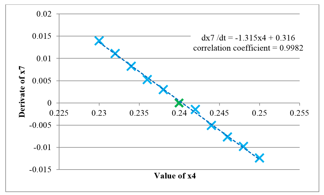
For each input or state, Bladed then makes a series of perturbations of increasing magnitude either side of the equilibrium point. The value of the state or input is artificially increased or decreased, the system is solved with these edited values and the state derivatives and outputs are recorded. The number of perturbations and the maximum perturbation magnitude can be defined by the user.

The elements of the matrices \(\bmatrix{A}\), \(\bmatrix{B}\), \(\bmatrix{C}\) and \(\bmatrix{D}\) can then be derived by performing a linear regression of the state derivative against the input or state value at all its perturbed values and its equilibrium value. The gradient of the linear regression gives the value of the element. If the correlation coefficient is less than the minimum correlation coefficient, then the relationship is considered void, and a zero value is given to the element.

Figure 1: Example linear regression calculating element \(\bmatrix{A}_{7,4}\) with a value of -1.315, with a correlation coefficient of 0.9982. The equilibrium point is shown in green

Last updated 02-08-2024