Integrators

Bladed offers several methods for time integration of the resulting dynamic equations that determine the evolution of the states (degrees of freedoms) of the non-linear wind turbine system, i.e. structural and aerodynamic states as well as other states originating from e.g. the turbine controller. Integrators are classified as either fixed step or variable step depending on whether the integrator time step may change during the simulation. A variable step integrator is practical as the time step changes dynamically in order to maintain a specified solution accuracy. However, some of the fixed step integrator methods are much faster at integrating systems with high frequency states such as multi-part blade models.

The different integrator types and their recommended usage are discussed in this section. The integrator type is selected in the Integrator settings screen.

Figure 1: Numerical integration involves computing an approximate numerical value for the area under the curve represented by the function \(f(x)\) and denoted as \(S\).

Variable step integrators

Runge-Kutta

The only variable step integrator in Bladed is a 4/5th order Runge-Kutta integrator (Kreyszig, 2006). This default setting is generally the best option for turbine models where each blade is modelled as a single finite element body.

For multi-part blade simulations or floating turbines with an explicit mooring line model, a fixed step integrator should be considered to improve the simulation speed.

Fixed step integrators

Various fixed step integrators are available in Bladed, as it appears when selecting Fixed step integrator for the Method parameter in the Integrator settings screen.

For all methods, a fixed integrator step size must be specified by the user in terms of the Time step input parameter. The time step parameter is important as it offers a trade off between simulation run time and solution accuracy. Generally speaking, a larger step size results in a faster simulation but can lead to lower results accuracy. Likewise, in general a smaller step size reduces simulation speed but improves accuracy. For implicit fixed step integrators a larger step size could also increase the number of iterations required for convergence of the solution thereby slowing down the calculation run time. It is necessary to ensure that the simulation accuracy is not excessively degraded by choosing too large a step size. In general, this may be checked by carrying out a reference simulation with a reduced step size (for example half the original step size) and check that the results in the relevant frequency range do not differ significantly.

The Newmark-\(\beta\) and Generalised-\(\alpha\) integrators described below are implemented in Bladed to allow efficient simulation of stiff structural systems that includes states with frequencies in a wider range. An example of this is a wind turbine model including the multi-part blade model.

Fixed step Newmark-\(\beta\) methods

The fixed step Newmark-\(\beta\) integrators (Newmark, 1959) use the Newmark-\(\beta\) difference scheme for discretising 2nd order states (structural states), while the remaining 1st order states (aerodynamic states, generator and so on) are discretised using the trapezoidal method. These integrators allow accurate integration of high frequency modes at larger time steps as long as the high frequency modes are well damped.

The Newmark-\(\beta\) algorithm is defined by the \(\bscalar{\beta}\) and \(\bscalar{\gamma}\) parameters that must be specified by the user in terms of the Beta and Gamma input parameters in the Integrator settings screen. With certain parameter settings \(\bscalar{\beta} \geq 0.25,\ \ \bscalar{\gamma} = 0.50\), the Newmark-\(\beta\) algorithm are unconditionally stable (i.e. stable regardless of step size) for linear systems, which results in good stability of the non-linear wind turbine system.

The recommended default settings \(\bscalar{\beta} = 0.25,\ \ \bscalar{\gamma} = 0.50\) result in the constant average acceleration method that is unconditionally stable for linear systems. In this case the acceleration is assumed to be constant over each time step and equal to the average of the values at the beginning and end of the time step.

However, when integrating a non-linear wind turbine system, the system can become unstable even with a moderate time-step size. Such instabilities are generally caused by erroneous blow up of high frequency modes, which in fact have only minor effect on the simulation results when stable. To achieve stability in such cases, it is common practice (and usually sufficient) to add structural damping on the high frequency blade and tower modes as described in the Flexibility screen . In particular, this is true for wind turbine models including the multi-part blade model.

Alternatively (or as a supplement), stability can be achieved by adding algorithmic damping (numerical damping) to the system by selecting the \(\bscalar{\gamma}\) parameter so that \(\bscalar{\gamma} > 0.5\), in which case it is recommended to adjust the \(\bscalar{\beta}\) parameter according to the formula \(\bscalar{\beta} = 0.25 (\bscalar{\gamma} + 0.5)^2\). For example, the parameter settings \(\bscalar{\beta} = 0.26, \bscalar{\gamma} = 0.52\) result in a method that is approximately equal to the constant average acceleration method but adds a small amount of algorithm damping to the system. It is emphasised that the algorithmic damping increases by the step size and occurs for both low and high frequency modes, which generally degrades the solution accuracy.

The integrator method is available in two different variants based on explicit and implicit formulations of the Newmark-\(\beta\) algorithm. It is recommended to use the latter, which generally produces more accurate results and allows using a larger step size (see also Bladed 4.11 release notes, November 2020). For both variants, the end state of a time step is estimated in an initial predictor step, but while the explicit variant accepts this estimate as the resulting end state, the implicit variant improves the accuracy in a number of corrector steps based on the iterative Newton-Raphson method applied to the system of dynamic equations. The convergence criteria for the Newton-Raphson iteration are based on an absolute error measure of the 1st and 2nd order states:

\[ \begin{align} & {\max_{i}\ \ }\frac{{\Delta \bvector{p}}_{i}}{{\bscalar{\epsilon}_{\bvector{p}}}_{i}} < \bscalar{T} \quad \textrm{for} \: 1^{st} \: \textrm{order states} \label{eq:con_crit_1} \\ & {\max_{i}\ \ }\frac{{\Delta \bvector{q}}_{i}}{{\bscalar{\epsilon}_{\bvector{q}}}_{i}} < \bscalar{T} \quad \textrm{and} \quad {\max_{i}\ \ }\frac{\bvector{r}_{i}}{{\bscalar{\epsilon}_{r}}_{i}} < \bscalar{T} \quad \textrm{for} \: 2^{nd} \: \textrm{order states} \label{eq:con_crit_2} \end{align} \]

where \({\Delta \bvector{p}}_{i}\) denotes the increments of the 1^st order states, \({\Delta \bvector{q}}_{i}\) denotes the increments of the 2^nd order states, while \(\bvector{r}_{i}\) denotes the residual forces conjugate to the 2^nd order states \(\bvector{q}_{i}\). The increments and the residuals are normalised using a set of epsilon values (absolute tolerances) \({\bscalar{\epsilon}_{\bvector{p}}}_{i}\), \({\bscalar{\epsilon}_{\bvector{q}}}_{i}\) and \({\bscalar{\epsilon}_{r}}_{i}\) that represent a set of sufficiently small numbers specified internally according to the expected order of magnitude of the state, possibly using some input parameters. The resulting convergence criterion is controlled by the tolerance multiplier denoted as \(\bscalar{T}\) that must be specified by the user in terms of the Tolerance multiplier input parameter with a recommended and default value of 1. If the convergence criterion is not met within 4 iterations (8 iterations if \(\bscalar{T}\) < 1), the step is rejected, and a half-sized re-step is requested. This process may continue resulting in a further step size reduction until the trial step size is close to the minimum allowable step size of 0.001 ms in which case the simulation terminates in an error state. So, although the implicit variant of the Newmark-beta method is categorised as a fixed step integrator it has also some variable step capabilities. The set of epsilon values for the state values and the residuals are output to the Software performance data group for each state in case that the Software performance option is selected in calculation outputs. In addition, this data group includes detailed information of the number of step reductions for each state caused by the integrator and the model (for example due to stick-slip phenomenon).

A key parameter for the Newmark-beta methods is the step size with default values of 5 ms and 20 ms for the explicit and the implicit variants, respectively. However, as described above, the actual step size for the implicit variant of the integrator may be reduced dynamically in order to ensure that the convergence criterion of the equilibrium iterations is fulfilled for all steps. In fact, this functionality may lead to a situation where the actual step size is significantly smaller than the specified step size, in which case a warning message is issued saying that it is recommended to reduce the specified step size. The actual step size and the corresponding normalised stepping frequency are output to the Simulation step sizes data group in case that the Software performance option is selected in the Calculation Output screen.

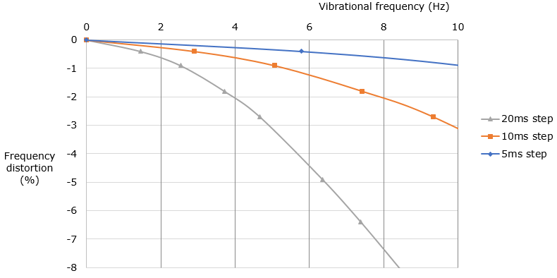
It is important to note that the solution accuracy depends significantly on the actual step size. A useful measure of the solution accuracy is given by the frequency distortion that is defined as the percentage difference between simulated and real vibration frequency of a dominant mode. For the default parameters settings \(\bscalar{\beta} = 0.25,\ \ \bscalar{\gamma} = 0.50\), a rule-of-thumb estimate of the frequency distortion is shown in the graph below as a function of the vibration frequency for three different step sizes (a negative value indicates that the simulated frequency is smaller than the real frequency). It is emphasised that the variation of the frequency distortion is generally different for other parameter settings.

Figure 1: Frequency distortion as a function of vibrational frequency for various step sizes.

Fixed step Generalised-\(\alpha\) method

The fixed step Generalised-\(\alpha\) integrator (Chung and Hulbert, 1993) is based on an extension of the Newmark-\(\beta\) difference scheme for discretising 2nd order states, while the 1st order states are discretised using the trapezoidal method. The integrator method is available in an explicit variant only and has a default step size of 5 ms. The integrator method applies damping to high frequency states whilst minimising the damping applied to low frequency states. The level of damping applied is controlled by the spectral radius at infinite frequency parameter. Adding damping in this fashion is desirable as the erroneous high frequency instabilities are avoided without significantly degrading the solution accuracy at lower frequencies.

Fixed step Runge-Kutta and Midpoint methods

These integrators offer lack the practicality of variable step Runge-Kutta and rarely offer performance benefits compared to Newmark-\(\beta\) and Generalised-\(\alpha\) integrators as the latter are better designed for structural systems. The Midpoint method is a 2nd order Runge-Kutta algorithm, which is the integrator that is used in real time Hardware Test simulations in versions 4.7 and earlier. The Runge-Kutta 4th order method is the classical Runge-Kutta method, which is widely used for numerical integration of ordinary differential equations.

Last updated 29-08-2024