The Ideal Rotor and Effects of Wake Rotation

By application of axial momentum theory, the induced velocity caused by the rotor can be calculated in the axial direction as well as the tangential direction. The induced velocity influences the relative flow speed at the rotor plane and thereby the aerodynamic loads calculated by the blade element theory. Traditionally, the induced velocity in the axial direction is expressed in terms of the axial induction factor \(\bscalar{a}\) as \(\bscalar{a V_0}\), where \(\bscalar{V_0}\) is the (axial) flow speed of the undisturbed flow. According to the axial momentum theory, including the application of Bernoulli’s equations, the resulting axial flow speed at the rotor plane then becomes \(\bscalar{V_0 (1-a)}\), while the flow speed in the wake becomes \(\bscalar{V_0 (1-2a)}\).

Similar to the axial induction factor, the tangential flow speed at a certain radius \(\bscalar{r}\) is traditionally expressed in terms of the tangential induction factor \(\bscalar{a'}\) as \(\bscalar{a' \Omega}\), where \(\bscalar{\Omega}\) is the rotor speed. According to simple momentum theory the rotational flow speed in the wake becomes \(\bscalar{2 a' \Omega r}\). Figure 1 shows an annular element of fluid as it passes the rotor. The flow speed at various points is shown:

• the undisturbed flow far upstream from the rotor,

• at the rotor plane,

• far downstream from the rotor.

Figure 1: Annular blade element (annulus) at radius \(\bscalar{r}\) with the flow velocities calculated from momentum theory at three locations: (a) undisturbed flow far upstream (b) at the rotor plane (c) far downstream of the rotor.

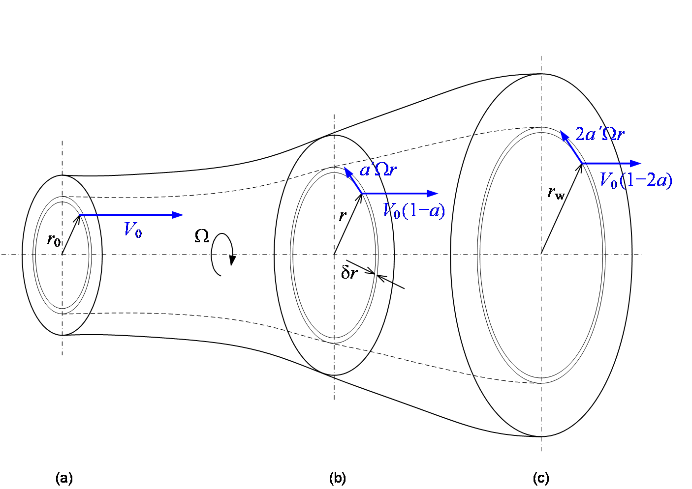
The following relationship considers the control volume indicated in Figure 1, which means that the cross-section area of the control volume at the rotor plane is \(\bscalar{\delta A} = \bscalar{2 \pi r \delta r}\), corresponding to the mass flow (\(\bscalar{\dot{m}}\))

\[ \begin{equation} \bscalar{\delta \dot{m}} = \bscalar{\rho V_0 (1-a) \delta A} = \bscalar{2 \pi \rho V_0 (1-a) r \delta r} \end{equation} \]

According the fundamental momentum theory, the resulting thrust (\(\bscalar{T}\)) and torque (\(\bscalar{Q}\)) on the control volume can be expressed as

\[ \begin{flalign} \bscalar{\delta T} &= \bscalar{2 a V_0 \delta \dot{m}} \\[1ex] \bscalar{\delta Q} &= \bscalar{2 a' \Omega r^2 \delta \dot{m}} \end{flalign} \]

The corresponding aerodynamic power (\(\bscalar{P}\)) then becomes

\[ \begin{equation} \bscalar{\delta P} = \bscalar{\Omega \delta Q} \end{equation} \]

In numerical computations it is convenient to express the axial and tangential induction directly in terms of the induced velocity components \(\bscalar{v_n}\) and \(\bscalar{v_t}\) rather than the induction factors \(\bscalar{a}\) and \(\bscalar{a'}\). The induced velocity components are therefore introduced as

\[ \begin{flalign} \bscalar{v_n} &= \bscalar{-a V_0} \\[1ex] \bscalar{v_t} &= \bscalar{-a' r \Omega} \end{flalign} \]

The final relations for thrust and torque can then be expressed as

\[ \begin{flalign} \bscalar{\delta T} &= \bscalar{-2 v_n \delta \dot{m}} \\[1ex] \bscalar{\delta Q} &= \bscalar{-2 v_t r \delta \dot{m}} \end{flalign} \]

Last updated 30-08-2024