IAG Model

The IAG model was developed based on the work from Bangga, 2020 which combined the first order terms based on the Beddoes-Leishman type model (Leishman, 1989a) with the second order terms based on the Snel type model (Snel, 1997). Several improvements were made to enhance the accuracy of the first and second order terms. The first order terms of the IAG model were transformed into a state-space representation in a recent work (Bangga, 2023), also regarded as the second generation. Here, some changes were introduced compared to the original model. The second generation IAG model (Bangga, 2023) is ultimately implemented in Bladed. This model consists of 5 states and is deemed most suitable for deep stall calculations when the angle of attack is large.

The modelling strategy of the first order terms is divided into several aerodynamic states: (1) attached flow state, (2) separated flow state and (3) vortex lift state. The following equations describe the IAG model.

The attached flow solutions are represented by two ordinary differential equations (ODEs) which are comparable to the deficiency functions

\[ \begin{flalign} \bscalar{& \left( \dfrac{c}{2V} \right){\dot{x}_{1}}(t) = b_{1}A_{1}\alpha_{n}^{3\text{/}4} - \left\lbrack b1 + \left( \dfrac{c\dot{V}}{2V^{2}} \right) \right\rbrack x_{1}(t) } \\[1ex] \bscalar{& \left( \dfrac{c}{2V} \right){\dot{x}_{2}}(t) = b_{2}A_{2}\alpha_{n}^{3\text{/}4} - \left\lbrack b2 + \left( \dfrac{c\dot{V}}{2V^{2}} \right) \right\rbrack x_{2}(t) } \end{flalign} \]

Here, \(\bscalar{x_{1,2}(t)}\), \({\bscalar{\dot{x}_{1,2}}(t)}\) and subscript \(\bscalar{n}\) represent the state of the ODEs, the state derivative of the ODEs and the sampling at a particular time instance, respectively. As suggested in Hansen, 2004, the added mass term \(\bscalar{c\dot{V}/(2V^{2})}\) is added to include the effects for varying wind speed in wind turbine cases. The effective angle of attack is calculated using:

\[ \begin{equation} \bscalar{ \alpha_{e_{n}} = \alpha_{n}^{3\text{/}4}\left( 1 - A_{1} - A_{2} \right) + x_{1}(t) + x_{2}(t) } \end{equation} \]

with \(\bscalar{\alpha_{n}^{3\text{/}4}}\) representing the angle of attack sampled at the quarter chord position. The circulatory normal force and impulsive effect (optional) can be obtained respectively using:

\[ \begin{flalign} \bscalar{& C_{N_{n}}^{C} = \dfrac{dC_{N}^{st}}{d\alpha}\sin\left( \alpha_{e_{n}} - \alpha_{0}^{st} \right) } \\[1ex] \bscalar{& C_{N_{n}}^{I} = 0.75\dfrac{4c}{V}\dot{\alpha_{n}} \phi_1^{impulsive} \phi^{damping} , } \end{flalign} \]

which yields the total contribution of the attached flow component as \(\bscalar{C_{N_{n}}^{P} = C_{N_{n}}^{C} + C_{N_{n}}^{I}}.\) Note that sinusoidal assumption is applied on the circulatory component to better capture high angle of attack behaviour as introduced in Bangga, 2023.

The next set of ODE is used to determine the time-lagged pressure response of the normal force

\[ \begin{equation} \bscalar{ \left( \dfrac{c}{2V} \right)T_{p}{\dot{x}_{3}}(t) = - x_{3}(t) + C_{N_{n}}^{P}, } \end{equation} \]

to calculate the delayed angle of attack

\[ \begin{equation} \bscalar{ \alpha_{f_{n}} = \alpha_{0}^{st} + \left( \dfrac{x_{3}(t)}{dC_{N}^{st}\text{/}d\alpha} \right). } \end{equation} \]

Here \(\bscalar{\alpha_{0}^{st}}\) represents the zero normal force angle of attack obtained from the static viscous polar data. By using the inverse of the Kirchhoff equation, the position of the separation point at \(\bscalar{\alpha_{f_{n}}}\) can be determined by:

\[ \begin{equation} \bscalar{ f_{n} = \left( 2\sqrt{\dfrac{C_{N_{n}}^{st}}{ \dfrac{dC_{N}^{st}}{d\alpha} \sin\left( \alpha_{f_{n}} - \alpha_{0}^{st} \right)}} - 1.0 \right)^{2}.} \end{equation} \]

The location of the separation point is further delayed by the fourth ODE

\[ \begin{equation} \bscalar{ \left( \dfrac{c}{2V} \right)T_{f}{\dot{x}_{4}}(t) = - x_{4}(t) + f_{n}, } \end{equation} \]

The unsteady viscous normal force can be reconstructed using a modified Kirchhoff equation

\[ \begin{equation} \bscalar{ C_{N_{n}}^{f} = \dfrac{dC_{N}^{st}}{d\alpha}\left( \dfrac{1 + \sqrt{x_{4}(t)}}{2} \right)^{2}\sin\left( \alpha_{e_{n}}\, - \,\alpha_{0}^{st} \right) + \, C_{N_{n}}^{I}. } \end{equation} \]

The last term to consider is the vortex lift effect due to the presence of the leading edge vortex as

\[ \begin{equation} \bscalar{ \left( \dfrac{c}{2V} \right)T_{v}{\dot{x}_{5}}(t) = - x_{5}(t) + \left( \dfrac{c}{2V} \right)T_{v}\dot{C_{V_{n}}}, } \end{equation} \]

with \(\bscalar{x_{5}(t)}\) specifying the normal force due to the vortex lift effect, which equals to \(C_{N_{n}}^{V}\) in the indicial representation (Bangga, 2020). To solve this equation, information about the rate of change of \(\bscalar{C_{V_{n}}}\) is needed. To do so, by applying a chain rule, a time derivative of \(\bscalar{C_{N_{n}}^{V}}\) is calculated as:

\[ \begin{equation} \bscalar{ {\dot{C}_{V_{n}}} = \dfrac{dC_{N}^{st}}{d\alpha}{\dot{\alpha}_{e_{n}}}\left( 1 - \dfrac{1}{4}\left( 1 + \sqrt{x_{4}(t)} \right)^{2} \right) - \dfrac{1}{4}C_{N_{n}}^{C}\left( 1 + \sqrt{x_{4}(t)} \right)\dfrac{{\dot{x}_{4}}(t)}{\sqrt{x_{4}(t)}}. } \end{equation} \]

This equation is only applied when there is a dynamic vortex state being active, otherwise \(\bscalar{{\dot{C}_{V_{n}}} = 0}\). The vortex state itself is defined when \(\bscalar{x_{3}(t)}\) is greater/smaller than the critical normal force:

\[ \begin{equation} \bscalar{C_{N}^{CRIT}} = \begin{cases} C_{N}^{MAX} & \text{if \quad Positive\ Stall} \\[1ex] C_{N}^{MIN} & \text{if \quad Negative\ Stall} \end{cases} \end{equation} \]

which refers to the maximum normal force (or minimum depending on the case) obtained from the static data. Another important consideration to activate \({\dot{C}_{V_{n}}}\) only during the upstroke motion. This implies that this is active (“Vortex state active”) only when the following conditions are met (for positive stall):

\[ \begin{equation} \bscalar{ \text{Upstroke} \quad \text{\&} \quad x_{3}(t) > C_{N}^{CRIT} \quad \text{\&} \quad 0 < \tau_{v_{n}} < T_{vl}. } \end{equation} \]

The upstroke state can be determined by \(\bscalar{ \Delta\alpha_{n}}\), but this will be different when the case being considered is positive stall (\(\bscalar{\Delta\alpha_{n} > 0}\)) or negative stall (\(\bscalar{\Delta\alpha_{n} < 0}\)). A positive stall case can be identified when \(\bscalar{x_{3}(t) \geq 0}\), while a negative stall case may be detected when \(\bscalar{x_{3}(t) < 0}\). For the backwinded case (when \(\bscalar{\text{|}\alpha\text{|}}\) is greater than \(\bscalar{90\degree{}}\)), the definition of upstroke is flipped. Now, the non-dimensional vortex time may be calculated using

\[ \begin{equation} \bscalar{\tau_{v_{n}}} = \begin{cases} \tau_{v_{n - 1}} + 0.45\dfrac{\Delta t}{c}V; & \text{if}\quad\text{Vortex\ state\ active} \\[1ex] \tau_{v_{n - 1}}\exp\left( - \dfrac{\Delta t}{c}V \right); & \text{otherwise} \end{cases} \end{equation} \]

For very large angle of attack approaching \(\bscalar{90\degree{}}\), it is assumed that the vortex lift effect vanishes. Therefore, the value is slowly relaxed towards zero from \(\bscalar{45\degree{}}\) to \(\bscalar{75\degree{}}\) using a simple linear function. This consideration is based on the fact that lift generally increases again after stall up to a full flow separation at around \(\bscalar{60\degree{}}\), see e.g. Sheldahl, 1981 and Garbaruk, 2009.

The final equation for the dynamic normal force coefficient is obtained from \(\bscalar{C_{N_{n}}^{f}}\) and \(\bscalar{\bscalar{C_{N_{n}}^{V}}}\) and is defined as:

\[ \begin{equation} \bscalar{C_{N_{n}}^{dyn} = C_{N_{n}}^{f} + C_{N_{n}}^{V}}. \end{equation} \]

The dynamic response of the chordwise aerodynamic force is simply obtained from:

\[ \begin{equation} \bscalar{C_{T_{n}}^{dyn} = C_{T_{n}}^{st} (\alpha_{f_{n}})}, \end{equation} \]

which allows one to calculate the dynamic lift coefficient response according to:

\[ \begin{equation} \bscalar{C_{L_{n}}^{dyn} = C_{N_{n}}^{dyn} \cos \alpha_n + C_{T_{n}}^{dyn} \sin \alpha_n }. \end{equation} \]

Note that this formulation is different with the description of Bangga, 2023 due to the definition of chordwise force being positive towards the leading edge while it is defined otherwise in Bangga, 2023.

The calculation for drag coefficient is done by applying the following relation:

\[ \begin{equation} \bscalar{ C_{D_{n}}^{dyn} = C_{D_{n}}^{st} + \left( \alpha_{n} - \alpha_{e_{n}} \right)C_{N_{n}}^{C} + \left( C_{D_{n}}^{st} - C_{D_{0}}^{st} \right)\left\lbrack \left( \dfrac{1 - \sqrt{x_{4}(t)}}{2} \right)^{2} - \left( \dfrac{1 - \sqrt{f^{st}}}{2} \right)^{2} \right\rbrack + x_{5}(t)\sin\alpha_{n}. } \end{equation} \]

In the above equation, variables \(\bscalar{C_{D_{n}}^{st}}\), \(\bscalar{C_{D_{0}}^{st}}\) and \(\bscalar{f^{st}}\) represent the static value of drag coefficient, drag level at zero normal force angle of attack and static separation position, respectively. Furthermore, it is assumed that drag force shows strong hysteresis only near stall regime. Therefore, the magnitude of drag is returned to the static value once the angle of attack is greater than \(\bscalar{30\degree{}}\). This is done through a linear blending up to \(\bscalar{45\degree{}}\). Note that a sudden drag increase occurs during stall and this takes place at \(\bscalar{\text{|}\alpha\text{|} < 30\degree{}}\) for most aerofoils.

Lastly, pitching moment coefficient is calculated based on the following relations

\[ \begin{equation} \bscalar{ C_{M_{n}}^{dyn} = C_{M_{n}}^{f} + C_{M_{n}}^{V} + C_{M_{n}}^{C}, } \end{equation} \]

with \(\bscalar{C_{M_{n}}^{f}}\) determining the separated state behaviour and can be obtained from the static data at delayed angle of attack as

\[ \begin{equation} \bscalar{ C_{M_{n}}^{f} = C_{M}^{st}\left( \alpha_{f_{n}} \right), } \end{equation} \]

and the vortex lift term of the pitching moment being represented as

\[ \begin{equation} \bscalar{ C_{M_{n}}^{V} = - 0.2\left( 1 - \text{\ cos}\left( \dfrac{\pi\tau_{v}}{T_{vl}} \right) \right)C_{N_{n}}^{V}. } \end{equation} \]

The last term is modelled as an added mass instead, and is defined as:

\[ \begin{equation} \bscalar{ C_{M_{n}}^{C} = - \dfrac{\pi c{\dot{\alpha}_{n}}}{4V} \phi_2^{impulsive} \phi^{damping} . } \end{equation} \]

For backwinded aerofoil orientation (when \(\bscalar{\text{|}\alpha\text{|}}\) is greater than \(\bscalar{90\degree{}}\)), the sign of \(\bscalar{C_{M_{n}}^{C}}\) becomes positive. Similar as for the drag coefficient, the magnitude of the pitching moment is returned to the static value once the angle of attack is greater than \(\bscalar{30\degree{}}\) through a linear blending with the static data.

Lastly, Bladed user has a control to deactivate the impulsive contribution factor \(\bscalar{\phi_1^{impulsive}}\) for the normal force. Its value is unity if the impulsive effect is activated and zero otherwise. For this model, the moment impulsive contribution factor (\(\bscalar{\phi_2^{impulsive}}\)) behaves equally the same as \(\bscalar{\phi_1^{impulsive}}\). Regardless of the choice of setting the impulsive effect, a damping factor (\(\bscalar{\phi^{damping}}\)) is always applied which decreases the contribution for fully separated flow or when the rate of change of the angle of attack (\(\bscalar{\dot{\alpha}}\)) becomes large. The scaling is done through the following relationship:

\[ \begin{equation} \bscalar{ \phi^{damping} = \max \left[ 0,\left( 1 - 8 \left( \dfrac{\dot{\alpha} c }{2 U} \right)^3 \right) \right] x_4 } \end{equation} \]

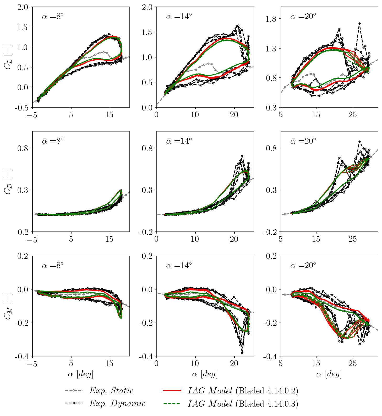
which is helpful to avoid potential instability of the solutions. Parameter \(\bscalar{\phi^{damping}}\) is added to the IAG model from Bladed 4.14.0.3 which results in a small deviation compared to Bladed 4.14.0.2 in the predictions of the lift and pitching moment coefficients, see Figure 1 for further details.

Figure 1: Dynamic force reconstruction of the pitching S809 airfoil at three different mean angles of attack (\(\bscalar{\bar{\alpha}}\)). The calculations are done at a reduced frequency \(\bscalar{k = 0.064}\) at an amplitude \(\bscalar{\Delta \alpha = 10\degree{}}\). Experimental data sets are obtained from Ramsay, 1995.

Last updated 30-08-2024