Calculating Coupled Modes

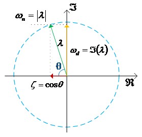
The Campbell diagram and blade stability analyses are analyses of the matrix \(\bmatrix{A}\) at each specified operating point. Each coupled mode corresponds to an eigenvalue and its eigenvector. Given a (complex) eigenvalue, \(\lambda\), of \(\bmatrix{A}\), Bladed reports the undamped frequency (\(\omega_n\)), damped frequency (\(\omega_d\)) and damping ratio (\(\zeta\)) according to Figure 1.

Figure 1: Argand Diagram

The uncoupled mode contributions to each coupled mode are determined by its eigenvector. If the coupled mode has contributions from second-order states (structural states), which are represented by two states in the state vector, then the displacement state is used to determine the contribution.

In their raw form, these eigenvector contributions represent the relative displacement of each mode and can be used to build up the coupled mode-shape. However, the contributions in the Campbell diagram have been normalised. This is done by modifying the matrix of eigenvectors such that each row and each column have a unit sum. This has the effect of increasing percentage contributions from modes with high mass and stiffness, which contribute very little in displacement but significantly in energy.

The phase of each contribution, \(\bscalar{\phi_{i}}\), is determined by the argument of the corresponding complex eigenvector element, \(\bscalar{v_{i}}\), i.e.

\[ \begin{align*} \bscalar{\phi_{i}} = \arctan\left( \frac{\operatorname{Im}\left( \bscalar{v_{i}} \right)}{\operatorname{Re}\left( \bscalar{v_{i}} \right)} \right). \end{align*} \]

Last updated 26-11-2024