Calculation Procedure

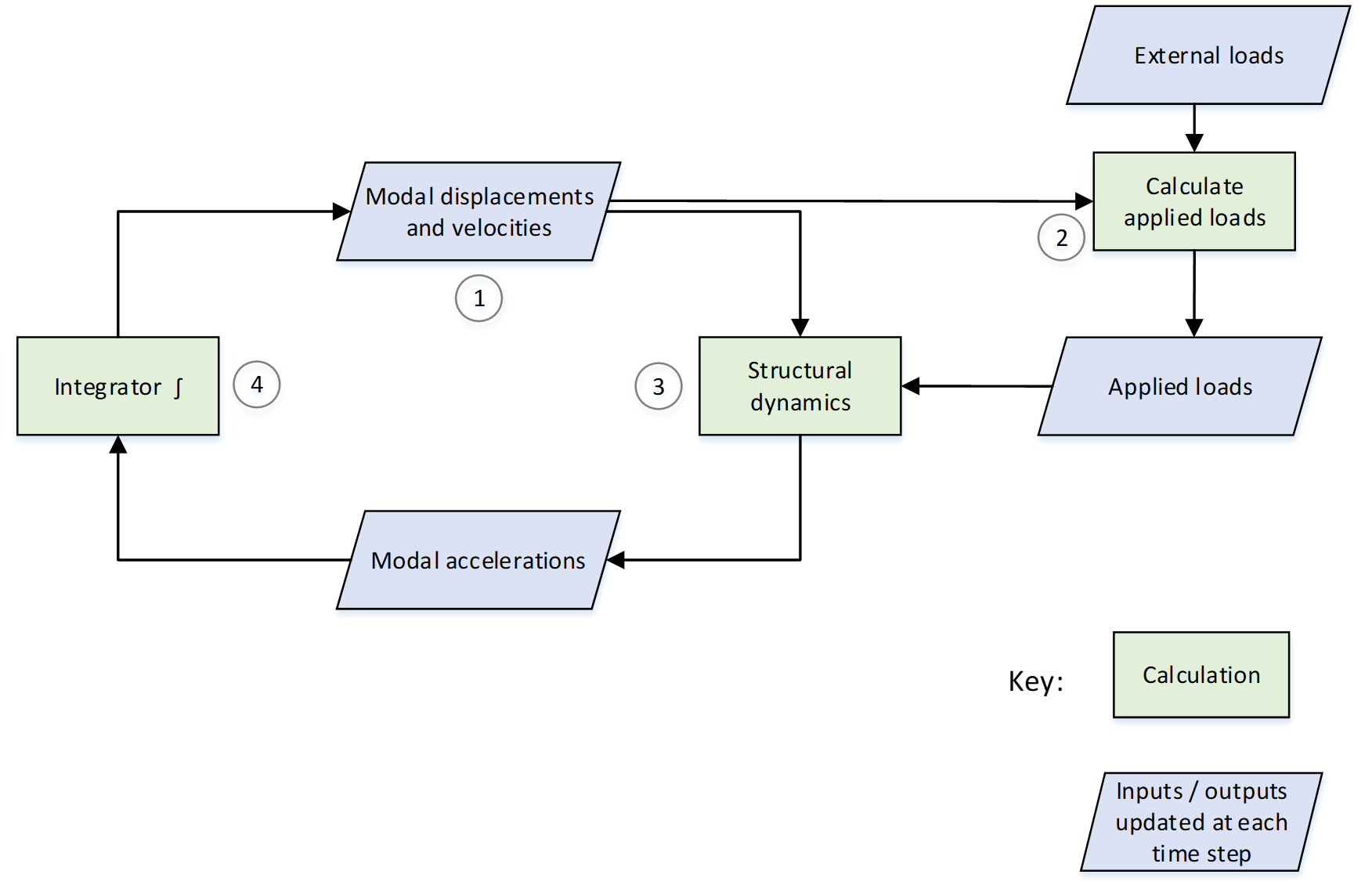
A schematic of the Bladed calculation to evaluate the structural response in the time domain is shown in Figure 1. The numbered steps below map directly to the numbered steps in the diagram.

1. Modal displacements and velocities (“state values”) are known at the start of the time step.

2. Applied loads are calculated based on the external loads and the state values. External loads applied at structural nodes are transformed into applied loads on the modes.

3. The structural dynamics equation \(\bmatrix{M}\ddot{\bvector{q}\ } + \bmatrix{C}\dot{\bvector{q}} + \bmatrix{K}\bvector{q} = \bvector{f}\) is solved in modal space to find the state accelerations \(\ddot{\bvector{q}}\), where

   • \(\bmatrix{M}\), \(\bmatrix{C}\), and \(\bmatrix{K}\) are the system modal matrices for mass, damping and stiffness respectively
   • \(\bvector{q}\), \(\dot{\bvector{q}}\), \(\ddot{\bvector{q}}\) and are the state displacements, velocities and accelerations respectively
   • \(\bvector{f}\) is the modal vector of externally applied forces on each state

4. The integrator uses the accelerations to find the state values at the next time step.

In most cases, applied loads depend partially on the nodal positions and velocities which are calculated from the state values. This is convenient as the states values are known at the start of each time step.

Figure 1: Schematic of calculation procedure of structural dynamics in time domain simulations

Last updated 30-08-2024