The Mann Model
This model is also referred to in the third edition of the IEC 61400-1 standard. It is based on a three-dimensional spectrum tensor representation derived from rapid distortion of isotropic turbulence by a uniform mean vertical velocity shear. The theory is given by (Mann, 1994) and (Mann, 1998). The method derives the spectral density for any three-dimensional wavenumber vector, and all three components of turbulence are then generated simultaneously by summing a set of such wavenumber vectors, each with the appropriate amplitude and random phase.
This is in many ways quite an elegant approach, but there are some practical limitations to be aware of. The summation requires a three-dimensional fast Fourier transform (FFT) to achieve reasonable computation time. The number of points in the longitudinal, lateral and vertical directions must be a power of two for efficient FFT computation. In the longitudinal direction, the number of points is determined by the length of time history required and the maximum frequency requested, and is therefore typically at least 1024. The maximum wavelength used is the length of the file (mean wind speed multiplied by duration), and the minimum wavelength is twice the longitudinal spacing of points (which is the mean wind speed divided by the requested frequency). In the lateral and vertical directions, a much smaller number of points must be used, perhaps as low as 32, depending on available computer memory. The maximum wavelength must be significantly greater than the rotor diameter, since the solution is spatially periodic, with period equal to the maximum wavelength in each direction. The number of FFT points then determines the minimum wavelength in these directions. With a realistic number of points, the resulting turbulence spectra are deficient at the high frequency end. (Mann, 1998) suggests that this is realistic, because it represents averaging of the turbulence over finite volumes of space which is appropriate for practical engineering applications. Bladed will report the loss of turbulence intensity due to this effect, so if a certain turbulence intensity is requested for a simulation, the actual turbulence intensity will be slightly lower due to a loss of high frequency variations.
Note also that the time histories at each grid point may have individual spectra and variances which can differ from one point to another. This may well be realistic of course, but it means that if the spectrum or variance is computed at any single point, for example at the hub position, the result may again be a little different from the expected value.
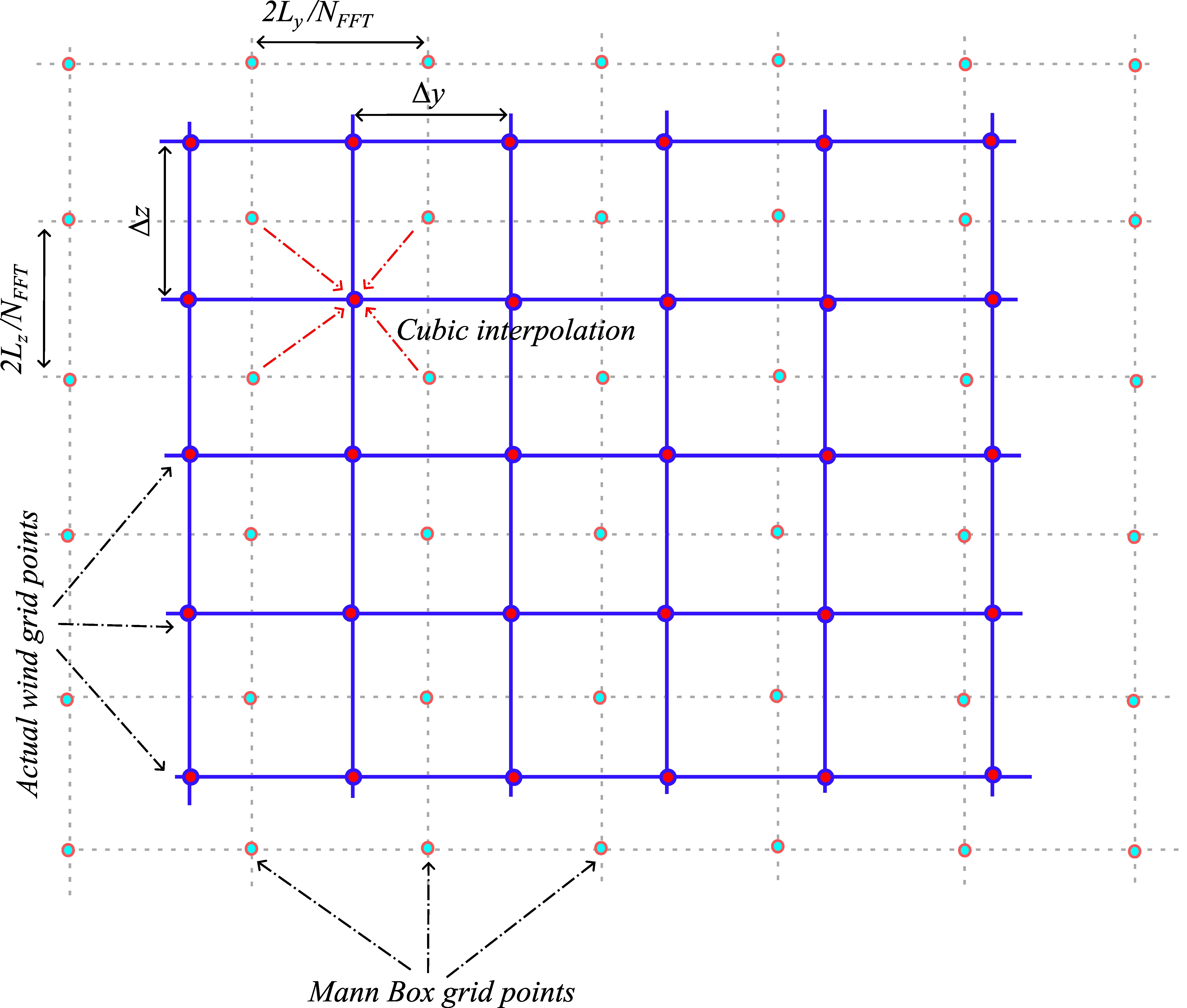
The Mann uniform shear turbulence model is generated based on the FFT points and outputted at the grid points specified by the user. This is illustrated in Figure 1 that shows the grids associated with the Mann turbulence generation and the actual grids written in the wind file (.wnd file). Total domain lengths in lateral and vertical directions are represented by \(L_y\) and \(L_z\) and the corresponding grid points \(N_y\) and \(N_z\), respectively. The Mann box itself will be discretized by the same FFT points in both directions. Note that the Mann box grid resolution in lateral direction is \(2L_y/N_{FFT}\). A factor of 2 shows because a half of the FFT points is required for calculating the spectral tensor components with negative wave numbers, and a half of it is used for the positive wave numbers. The same is also true for the vertical component. The turbulent fluctuations obtained from the Mann box calculations are then mapped onto the actual wind file grid by means of cubic interpolation.
Last updated 30-08-2024