Comparison against Analytical Solutions for a Two Degree of Freedom Aerofoil

In this articles the analytical flutter boundary for a 2 degree of freedom (DOF) aerofoil will be compared against an equivalent numerical model in Bladed.

Governing Equations

To test the basic functionality of the stability tool a comparison is carried out between an analytical solution of a two degree of freedom pitching and plunging aerofoil and the numerical solution in Bladed. Figure 1 shows an example of a 2D aerofoil that is attached to a linear \(K_h\) and a torsional \(K_{\phi}\) spring. The aerofoil is assumed to have a mass \(m\) which is located at a distance \(d\) from the spring mounting position also referred to as the elastic axis. Further the aerofoil has a rotational inertia \(J\).

Figure 1: Schematic of a 2DOF aerofoil. The red dot is the position of the aerodynamic centre and the yellow dot is the position of the centre of mass and inertia.

If one would assume flat-plate theory and fully steady aerodynamics, then the steady aerodynamic lift force and moment force can be described as:

\[ \begin{flalign} q_{\infty} &= \frac{1}{2} \rho U^2 \\[1ex] L &= 2 \pi \theta q_{\infty} S \label{eq:lift} \\[1ex] M &= 2 \pi \theta q_{\infty} e S U^2 \label{eq:moment} \end{flalign} \]

where:

• \(U\) is the relative wind speed at the aerofoil
• \(\rho\) is the air density
• \(e\) is the offset between the elastic and aerodynamic axis
• \(d\) is the offset between the elastic and mass axis
• \(q_{\infty}\) the dynamic pressure
• \(S\) the wing surface area
• \(\theta\) spring rotation angle
• \(h\) spring translational displacement

Then the equations of motion of the system are:

\[ \begin{equation} \left[\begin{array}{cc} m & -md \\ -md & J \end{array}\right] \left[\begin{array}{c} \ddot{h} \\ \ddot{\theta} \end{array}\right] + \left[\begin{array}{cc} K_h & 2 \pi \theta q_{\infty} \\ 0 & K_{\theta} - 2 \pi \theta q_{\infty} e \end{array}\right] \left[\begin{array}{c} h \\ \theta \end{array}\right] = \left[\begin{array}{c} 0 \\ 0 \end{array}\right] \label{eq:eqnmotion2dofaerofoil} \end{equation} \]

Further if the damping due to the motion of the aerofoil is included the lift force can be rewritten as:

\[ \begin{equation} L = 2 \pi q_{\infty} S \left( \theta - \left( \frac{\dot{h} + \dot{\theta}e}{U} \right) \right) \end{equation} \]

Substituting this into the equations of motion yields:

\[ \begin{equation} \left[\begin{array}{cc} m & -md \\ -md & J \end{array}\right] \left[\begin{array}{c} \ddot{h} \\ \ddot{\theta} \end{array}\right] + 2\frac{\pi q_{\infty}S}{U} \left[\begin{array}{cc} 1 & e \\ e & e^2 \end{array}\right] \left[\begin{array}{c} \dot{h} \\ \dot{\theta} \end{array}\right] + \left[\begin{array}{cc} K_h & 2 \pi \theta q_{\infty} \\ 0 & K_{\theta} - 2 \pi \theta q_{\infty} e \end{array}\right] \left[\begin{array}{c} h \\ \theta \end{array}\right] = \left[\begin{array}{c} 0 \\ 0 \end{array}\right] \label{eq:eqnmotion2dofaerofoilfinal} \end{equation} \]

Assuming a harmonic solution of the form \(h(t) = \ \widehat{h}e^{\lambda t}\) then an eigenvalue problem is formulated yielding to the characteristic equation

\[ \begin{equation} A\lambda^{4} + B\lambda^{2} + C = 0 \end{equation} \]

where:

\[ \begin{flalign} A &= mJ = m^2 d^2 \\[1ex] B &= K_h J + K_{\theta} - (md + me)2\pi q_{\infty}S \\[1ex] M &= K_h (K_{\theta} - 2\pi q_{\infty}Se) \end{flalign} \]

If the low frequency damping is included then the characteristic equations takes the form

\[ \begin{flalign} 0 &= A \lambda^4 + B \lambda^3 + C \lambda^2 + D \lambda + E \label{eqn:char} \\[1ex] A &= mJ = m^2 d^2 \\[1ex] B &= \frac{2\pi q_{\infty}S}{U} (me^2 + J) \\[1ex] C &= K_h J + K_{\theta} - (md + me)2\pi q_{\infty}S \\[1ex] D &= \frac{2\pi q_{\infty}S}{U} - (K_{\theta} - 2\pi q_{\infty}Se) \\[1ex] E &= K_h (K_{\theta} - 2\pi q_{\infty}Se) \end{flalign} \]

Equation \(\eqref{eqn:char}\) cannot be solved analytically and requires a numerical root finder. This is carried out using the numpy.roots() function in a Python script.

Comparison of Bladed to Analytical Solution for a Flat-Plate Aerofoil

A Bladed model is created representing a two degree of freedom aerofoil. Modelling this simple case in Bladed is relatively challenging as Bladed is not designed to model two-degree of freedom systems. The 2D aerofoil is therefore modelled as a 100 \(\bunit{m}\) blade with a uniform torsional and flapwise stiffness. The edgewise stiffness is kept a factor 5 above the flapwise stiffness to ensure that the first two blade modes are a flapwise and torsional mode. Further the mass and inertia is concentrated near the tip by using a split station at the last 1m of blade length. The first 99m of the blade is modelled with nearly zero mass and inertia. Finally, the first 99m of the blade uses an aerofoil with zeros as coefficients for lift, drag and moment coefficients. The last 1m of the blade is using a flat-plate aerofoil with \(C_l= 2 \pi \sin (\alpha)\).

To represent the bending/torsional stiffness of an equivalent single mass-spring system the following well-known cantilever deflection \(\delta\) and torsional rotation \(\theta\) formulas are used

\[ \begin{flalign} \delta &= \frac{FL^3}{3EI}, \\[1ex] \theta &= \frac{ML}{GJ}. \end{flalign} \]

The following variables are defined:

• \(M\), bending moment applied at the free end of the beam,
• \(L\), beam length,
• \(EI\), beam bending stiffness,
• \(F\), discrete force applied at the free end of the beam, and
• \(GJ\), torsional rigidity of the beam.

The equivalent spring constants then are:

\[ \begin{flalign} K_{t} &= \frac{3EI}{L^{3}}, \\[1ex] K_{\theta} &= \frac{GJ}{L}. \end{flalign} \]

Table 1 summarizes all the inputs to the model.

Table 1: Parameters used for flutter calculation

Parameter	Quantity	Unit
Rotational inertia	0.75	kgm
Mass	10	kg
Linear spring constant	30000	kg/m
Torsional spring constant	3000	kg/m
Centre of mass	45	% chord
neutral axis	25	% chord
Shear centre	25	% chord
Flapwise frequency	7.9	Hz
Torsional frequency	11.1	Hz

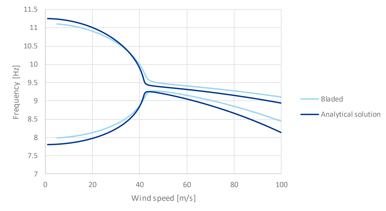
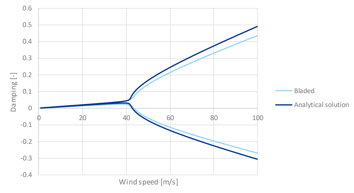
The results in Figure 2 and Figure 3 demonstrate a good match between the Bladed simulation and the analytical solution. In both cases the frequency branches merge around 43 m/s. At this same wind speed the damping of the torsional mode goes negative.

Figure 2: Comparison of analytical model against Bladed simulation outputs of blade mode frequency against wind speed for 2D aerofoil flutter problem.

Figure 3: Comparison of analytical model against Bladed simulation outputs of blade mode damping against wind speed for 2D aerofoil flutter problem.

Last updated 09-09-2024