LIDAR Sensor

Bladed allows a LIDAR (Light Detection And Ranging) sensor to be used to provide wind preview information to the external controller. A LIDAR sensor is a laser Doppler anemometer which sends out a laser beam and detects returning reflections from small particles or aerosols moving with the wind. Through the Doppler effect, the difference in frequency between outgoing and incoming signals gives a direct measure of the reflecting particle’s velocity component in the direction of the beam line.

LIDAR algorithm

The LIDAR beam is arranged to sample the velocity at a certain distance along the beam, either by focussing the beam at a certain distance in the case of a continuous-wave (CW) LIDAR, or by pulsing the beam and measuring the time interval between emitting the pulse and receiving a reflection. Reflections will be received from particles all the way along the beam, so by separating these according to the time interval since the pulse was emitted, velocities at different distances along the beam can be measured from each pulse.

Whether a CW or pulsed LIDAR is used, each measured velocity sample uses reflections from many particles, distributed within a volume of air in the vicinity of the focal point of a CW beam, or representing a range gate defined by certain band of reflection intervals in the case of a pulsed beam. This ‘volume averaging’ effect can be modelled by assuming that the measured velocity is representative of a volume of air centred on the focal point or the centre of the range gate. This is implemented in Bladed by means of a weighting function used to calculate a weighted average of actual velocities, resolved into the direction of the beam, at a series of points along the beam.

The weighting function for a pulsed LIDAR should be entered by the user. A typical weighting function might be given by $w(x) = (1 - |x|/d)^2$ for \(–d < x < d\), at a distance x from the mid-point of the range gate, where \(d\) is the half-width of the range gate. The weighting function for a continuous-wave LIDAR depends on the laser wavelength \(\lambda\), the lens area \(A\), and the distance \(R\) to the focal point see (Simley et al, 2011)

\[ \begin{equation} w(x) = \frac{R^{2}/(1 + c^{2})}{{(R + x)}^{2} + {(x/c)}^{2}} \end{equation} \]

where \(c = R \lambda / A\). laser wavelength \(\lambda\), the lens area \(A\), and the distance \(R\) to the focal point see (Simley et al, 2011)

\[ \begin{equation} w(x) = \frac{R^{2}/(1 + c^{2})}{{(R + x)}^{2} + {(x/c)}^{2}} \end{equation} \]

where \(c = R \lambda / A\).

Within Bladed, this is defined by default as a lookup table of 13 points centred on the focal point, distributed such that the shape of the weighting function is adequately represented out to 1% of its peak value.

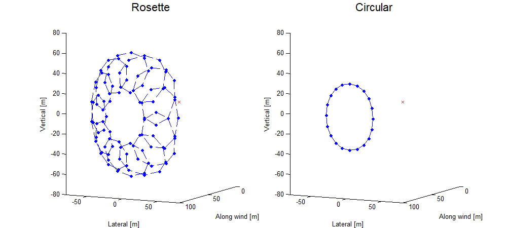
LIDAR scan patterns

The user can apply one of the pre-defined scanning techniques, fixed position, circular scanning or rosette scanning, see Figure 1. If the fixed scan pattern is selected the beam direction is coincident with the LIDAR axis.

The scan patterns are defined in terms of two angles \(\alpha\) and \(\beta\). These are defined relative to the LIDAR axis. Please consult the user manual for more details on the definition of the coordinate systems.

The number of samples per complete scan \(N_{s}\), should be specified by the user along with the sampling rate \(T_{s}\). The period of each scan is given by \(T = T_{s} \cdot N_{s}\).

For the circular scan, the user must specify a constant angle \(\alpha\) to the LIDAR axis centreline. At each sample interval time \(t = nT_{s}\) (where \(n\) is an arbitrary non-negative integer), the LIDAR beam direction is updated such that \(\beta = 2\pi t/T\)

For the rosette scan pattern, the user must specify the min and max angles \(\phi_{\min}\) and \(\phi_{\max}\) to the LIDAR axis centreline and the number of lobes \(N_{L}\). The following equations are used to determine the value of beam angles \(\alpha\) and \(\beta\).

\[ \begin{flalign} a_{1} &= (\phi_{\max} + \ \phi_{\min})/2 \label{rosettaScanEq1} \\[1ex] \omega_{1} &= \dfrac{2\pi}{T} \label{rosettaScanEq2} \\[1ex] \omega_{2} &= \dfrac{2\pi N_{L}}{T} \label{rosettaScanEq3} \\[1ex] y &= {a_{1}\cos}{\omega_{1}t} + {a_{2}\sin}{\omega_{2}t} \label{rosettaScanEq4} \\[1ex] z &= {a_{1}\sin}{\omega_{1}t} + a_{2}\sin{\omega_{2}t} \label{rosettaScanEq5} \\[1ex] \alpha &= \sqrt{y^{2} + z^{2}} \label{rosettaScanEq6} \\[1ex] \beta &= \arctan \left( \dfrac{z}{y} \right) \label{rosettaScanEq7} \end{flalign} \]

Figure 1: Examples of Rosette (left) and circular (right) scanning patterns created using one LIDAR beam. Rosette scan created using \(N_s=100\), \(N_L=12\), \(\varphi_{min}=15\degree\) and \(\varphi_{max}=45\degree\). Circular scan created using \(N_s=20\) and \(\alpha=20\degree\). Blue line with dots shows scan locations. LIDAR origin is (0,0,0) and focal beam length is 100.

Last updated 10-09-2024