Blade Element Method

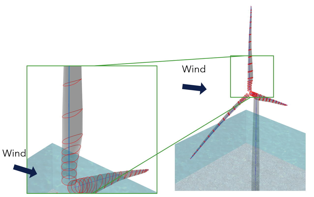
For computation of aerodynamic loads on a blade the standard approach is to discretise the blade into a series of elements spanning the length of the blade that adjoin at station nodes. Each station node defines the position of the blade section frame that describes the orientation and kinematics of the aerofoil cross-section. This then enables the computation of angle of attack by projecting the incident relative wind velocity at a blade section into the cross-section orientation and accounting for the direction of the chord line. This article describes how the blade inputs are transformed by the aerodynamics module to construct the blade section frame for the calculation of aerodynamic loading. A single rotor upwind turbine is used to explain the definition of the blade section as shown in Figure 1.

Figure 1: Picture of a single rotor upwind turbine. The blade is discretised into elements that lie on the blade neutral axis (blue line) and adjoin blade stations that are denoted by aerofoil cross-sections (red curves).

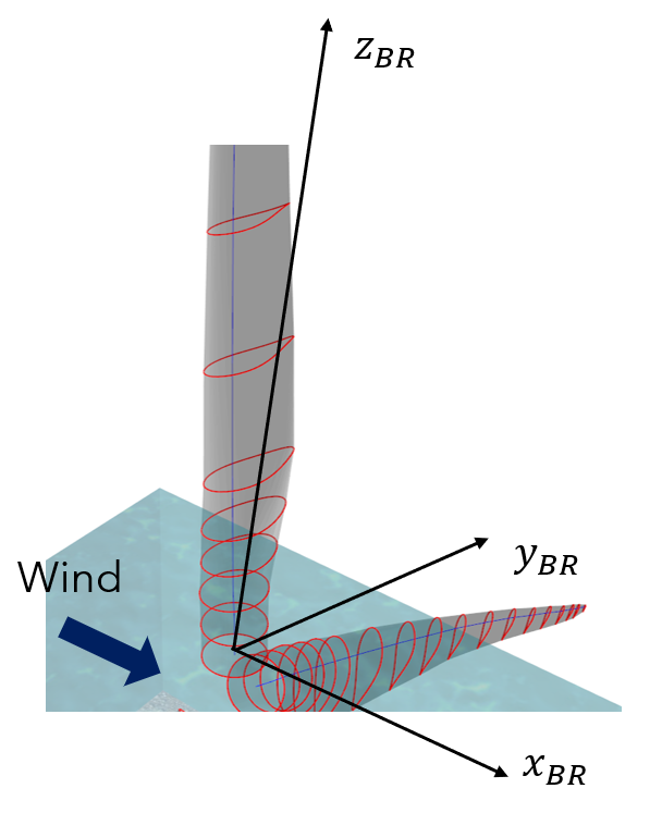
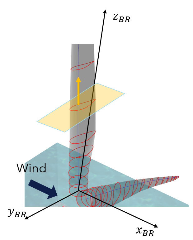
The starting point to define the orientation of the blade section frame is the blade root coordinate system shown in Figure 2. The blade root axes are used for the input of blade data such as the neutral axis, and aerodynamic twist.

Figure 2: Diagram of the blade root axes for blade 1 of the turbine.

Neutral Axis and Aerodynamic Twist

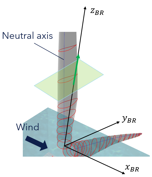
The neutral axis is defined relative to the blade root axes and defines a piecewise linear spline running along the span of the blade. Each point of the neutral axis defined by the user defines a blade station used for aerodynamic load computation. At each blade station a plane can be formed that is spanned by the axes \(x_{BR}\) and \(y_{BR}\) and coincident with a point along the neutral axis defined by the user. This plane is referred to as \(NA\) and is shown in Figure 3. Obviously, the axis \(z_{BR}\) will be normal to \(NA\).

Figure 3: Plane \(NA\) spanned by \(x_{BR}\) and \(y_{BR}\) and coincident with a point on neutral axis defined by user. The aerodynamic twist is defined in this plane.

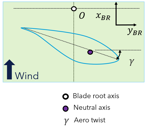
The aerodynamic twist defines a rotation of the blade aerofoil cross-section from the \(y_{BR}\) axis to the chord line. A positive rotation pushes the leading edge of the blade into the wind. This rotation is about the \(z_{BR}\) axis.

Figure 4: Plane spanned by \(x_{BR}\) and \(y_{BR}\) and coincident with a point on the neutral axis defined by user. The aerodynamic twist is defined in this plane.

Orientation of Blade Section

The tangent vector of the various linear segments of the spline are easily defined however this tangent vector to the spline is discontinuous at the joins of the piecewise linear segments. At the adjoining points the tangent vectors are averaged to create a "local" tangent vector \(\bvector{t}_s\) to the spline at the blade station. A plane \(BE\) is defined by a point on the neutral axis and the "local" tangent as shown in Figure 5.

Figure 5: The local tangent vector \(\bvector{t}_s\) (in yellow) to the neutral axis at the blade section that is normal to the plane \(BE\).

The orientation of the blade section is then defined by two rotations:

1. The first is the rotation of the aerodynamic twist \(\gamma\) about the \(z_{BR}\) axis. This creates an intermediate set of axes \((x_{BR}', y_{BR}', z_{BR}')\).
2. The second is a rotation of the vector \(z_{BR}'\) onto the local tangent vector \(\bvector{t}_s\).

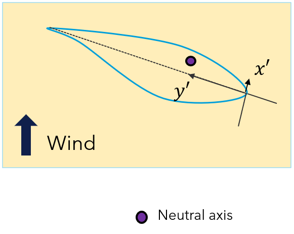
Finally, the position of the leading edge of the aerofoil cross section relative to the neutral axis is defined by the inputs \((x',y')\) as shown in Figure 6. This information is then used to define the orientation and the position of the aerofoil for the aerodynamic loading calculation. The directions \(('x,'y')\) are normal to the local tangent vector \(\bvector{t}_s\). The input x' defines the percentage of the chord distance the leading edge is positioned relative to the neutral axis in a direction normal to the chord line. The input y' defines the percentage of the chord the leading edge is positioned relative to the neutral axis along the chord line.

Figure 6: Position of leading edge of aerofoil relative to the neutral axis position in the blade section frame.

Last updated 07-08-2024