Flow Speed Components at an Aerofoil Section

Figure 1 shows a typical aerofoil section with the flow velocities as well as the aerodynamic loads shown as vectors. The relative flow velocity \(\bvector{W}\) is the vector sum of the undisturbed flow velocity \(\bvector{V_0}\), the apparent flow velocity \(\bvector{V_s}\) caused by the structural motion, and the induced velocity \(\bvector{v}\) accounting for the presence of the rotor. Expressed in the global inertial frame of reference, the relative flow velocity is therefore expressed by the following fundamental relationship

\[ \begin{equation} \bvector{W} = \bvector{V_0} + \bvector{V_s} + \bvector{v} \end{equation} \]

Figure 1: Aerofoil section with flow velocities and aerodynamic loads. The blade is pointing out of the paper and moves towards the right, while the flow is coming from below. Applies to clockwise rotors only. Blade tip pointing out of the page.

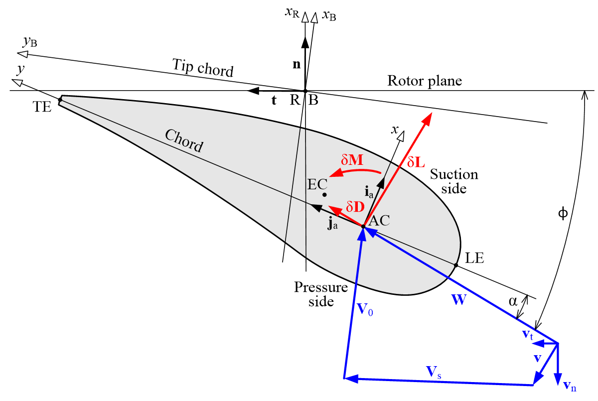
It is noted that the undisturbed flow velocity \(\bvector{V_0}\) is affected by several factors such as mean flow speed, flow direction, flow shear, turbulence, and possible tower “shadow” effects. The flow velocity \(\bvector{V_s}\) caused by the structural motion is opposed to the absolute structural velocity (\(\bvector{v_s}\)) defined, i.e.

\[ \begin{equation} \bvector{V_s} = \bvector{- v_s} \end{equation} \]

The structural velocity at the elastic axis is subsequently corrected for the offset between the aerodynamic centre at \(\bvector{x_{c/4}}\) and the elastic axis at \(\bvector{x_{ec}}\).

\[ \begin{equation} \bvector{V_s} = \bvector{-\left( v_s + \omega _B \times \left(x_{c/4} - x_{ec} \right) \right)} \end{equation} \]

With the induced velocity expressed in terms of the axial (normal) and tangential velocity components \(\bscalar{v_n}\) and \(\bscalar{v_t}\) introduced in the modelling of ideal rotor and effects of wake rotation, the induced velocity vector can be expressed as

\[ \begin{equation} \bvector{v} = \bscalar{v_n}\bvector{n} + \bscalar{v_t}\bvector{t} \end{equation} \]

where \(\bvector{n}\) and \(\bvector{t}\) are the base vectors defining the normal to the rotor plane and the tangent to the annulus as defined in Figure 1.

The aerodynamic loads acting on the control volume are described in terms of the lift force \(\bscalar{\delta L}\) and the drag force \(\bscalar{\delta D}\) indicated in Figure 1, where \(\bscalar{\alpha}\) denotes the angle of attack. The resulting local components of the aerodynamic load can then be expressed in the form

\[ \begin{flalign} \bscalar{p_x \delta z} &= \bscalar{\delta L \cos \alpha + \delta D \sin \alpha} \\[1ex] \bscalar{p_y \delta z} &= \bscalar{\delta D \cos \alpha - \delta L \sin \alpha} \end{flalign} \]

where \(\bscalar{p_x}\) and \(\bscalar{p_y}\) are the local components of the resulting aerodynamic load per unit length of the aerofoil. The forces are then rotated from the global frame into the axial (normal) and tangential components and combined with the relations for thrust and torque giving

\[ \begin{flalign} \bscalar{N_B p_n \delta z} &= \bscalar{-2 v_n \delta \dot{m}} \\[1ex] \bscalar{N_B p_t \delta z} &= \bscalar{-2 v_t \delta \dot{m}} \end{flalign} \]

where \(\bscalar{\delta \dot{m}}\) denotes the mass flow through the annulus. This quantity may be expressed as:

\[ \begin{equation} \bscalar{\delta \dot{m}} = \bscalar{N_B \dfrac{d \dot{m}}{dr} \delta r} = \bscalar{N_B \dot{m}' J \delta z} \end{equation} \]

where \(\bscalar{N_B}\) is the number of blades, and \(\bscalar{\dot{m}'} = \bscalar{\dfrac{\delta \dot{m}}{\delta r}}\) is the mass flow rate per unit length in the rotor plane, while \(\bscalar{J} = \bscalar{\dfrac{d r}{d z}}\) is a geometric parameter that can be derived from the structural model. For a rigid coned rotor with straight blades, the parameter \(\bscalar{J}\) equals cosine of the cone angle. The final fundamental momentum equilibrium equations for the annulus can then be derived as:

\[ \begin{flalign} \bscalar{v_n} &= \bscalar{-\dfrac{p_n}{2 J \dot{m}'}} \\[1ex] \bscalar{v_t} &= \bscalar{-\dfrac{p_t}{2 J \dot{m}'}} \end{flalign} \]

These equations are basically used for calculating the axial (normal) and tangential components of the induced velocity.

The mass flow at the rotor plane is expressed in terms of the yet unknown local convection velocity \(\bscalar{V_m}\) as \(\bscalar{\delta \dot{m} = \rho V_m \delta A}\), where \(\bscalar{\rho}\) is the air density and where \(\bscalar{\delta A}\) is the flow area defined as \(\bscalar{\delta A = 2 \pi r \dfrac{\delta r}{N_B}}\). Hence

\[ \begin{equation} \bscalar{\dot{m}'} = \bscalar{\rho V_m \dfrac{2 \pi r}{N_B}} \end{equation} \]

For ideal axial flow the convection velocity is identical to the velocity at the rotor plane (\(\bscalar{V_m = V_0 + v_n}\)) where \(\bscalar{V_0} = \left| \bvector{V_0}\right|\) is the undisturbed flow speed. In case \(\left| \bvector{V_0}\right|\) is not perpendicular to the rotor plane, the normal component is used and the convection velocity is therefore expressed in the more general form

\[ \begin{equation} \bscalar{V_m} = \bvector{n^T V_0} + \bscalar{v_n} \end{equation} \]

With the Glauert momentum theory described in Glauert, 1926a the corresponding convection velocity is expressed as

\[ \begin{equation} \bscalar{V_m} = \left| \bvector{V_0} + \bscalar{v_n} \bvector{n} \right| \end{equation} \]

The aerodynamic lift and drag forces as well as the aerodynamic moment acting on the blade element are modelled in terms of the lift, drag and moment coefficients \(\bscalar{C_L}\), \(\bscalar{C_D}\) and \(\bscalar{C_M}\) by the usual relationships

\[ \begin{flalign} \bscalar{\delta L} &= \bscalar{\dfrac{1}{2} \ \rho \ W_{xy}^2 \ C_L \ c \ \delta z} \\[1ex] \bscalar{\delta D} &= \bscalar{\dfrac{1}{2} \ \rho \ W_{xy}^2 \ C_D \ c \ \delta z} \\[1ex] \bscalar{\delta M} &= \bscalar{\dfrac{1}{2} \ \rho \ W_{xy}^2 \ C_D \ c^2 \ \delta z} \end{flalign} \]

with \(\bscalar{W_{xy}}\) being the magnitude of relative velocity component normal to local spanwise direction and \(\bscalar{c}\) being the local chord length of the aerofoil section.

Like in any BEM code, the aerofoil coefficients are determined from lookup tables. These can be interpolated based on thickness to chord ratio, Reynolds number, deployment angle and tip speed ratio. The latter could be used to include the effect of stall-delay near the root of the blade. No model for stall delay is implemented in the Bladed BEM code, thus it is required to pre-correct the tabulated aerofoil data for any 3D effects in advance by means of empirical corrections or 3D synthesized data (Hansen, 2015; Bangga, 2022).

Last updated 30-08-2024