Generation of Response Spectrum Compatible Accelerogram

The earthquake algorithm generates an accelerogram  \(\bscalar{\ddot{u}(t)}\) of duration \(\bscalar{T}\) secs. A high level summary of the algorithm is provided in Figure 1.

An acceleration time history is first created by generating a series of random phases and amplitudes. These are used to define the discrete Fourier transform of the characteristic earthquake shape. It is possible to use a specific set of phases using a seed thus ensuring repeatability of results. An arbitrary seed can be chosen.

Figure 1: Algorithm for creating an acceleration time series for an earthquake.

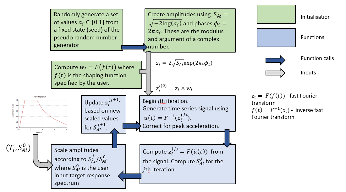
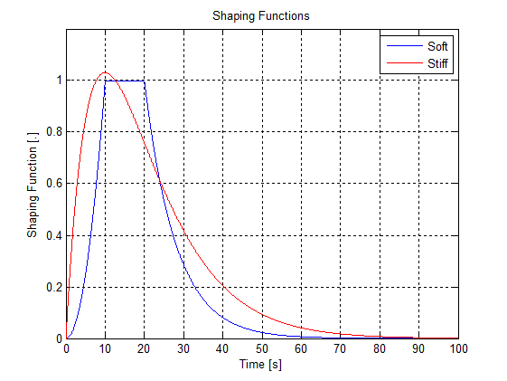
A shaping function is used to scale the amplitudes and the signal is passed through a low and high pass band filter to remove unwanted frequencies. The user can choose between an overall shape typical of stiff or soft soil properties. If stiff soils are specified, then the shaping function takes the form \(\bscalar{f(t)} = \bscalar{a_{1}}\bscalar{t}\bscalar{\exp}{( - \bscalar{a_{2}}\bscalar{t})}\). The parameters \(\bscalar{a_{1}} = 28/\bscalar{T}\) and \(\bscalar{a_{2}} = 10/\bscalar{T}\) are specified at run time such that the maximum scaling factor of \(\bscalar{f(t)}\) is 1 and the decay is complete by the end of the earthquake. If soft soils are specified, then the following equation is used

\[ \begin{equation} \bscalar{f(x)} = \left\{ \begin{aligned} \left( \frac{\bscalar{t}}{\bscalar{t_{1}}} \right)^{2}\ \ \ \ \ \ \ \ ,\ \ & \bscalar{0} < \bscalar{x} < \bscalar{t_{1}} \\ 1\ \ \ \ \ \ \ \ \ \ \ \ \ \ ,\ \ & \bscalar{t_{1}} < \bscalar{x} < \bscalar{t_{2}} \\ \exp\left\lbrack - \frac{\bscalar{c}\left( \bscalar{t} - \bscalar{t_{2}} \right)}{\bscalar{T} - \bscalar{t_{2}}} \right\rbrack,\ \ & \bscalar{x} \geq \bscalar{t_{2}} \\ \end{aligned} \right.\ \end{equation} \]

where \(\bscalar{t_{1}}\), \(\bscalar{t_{2}}\) and \(\bscalar{c}\) are user defined constants.

See Figure 2 for shaping function curves.

Figure 2: Shaping functions for soft and stiff soils. The curves were generated using the following inputs parameters: \(\mathbf{T = 100}\) s,\(\mathbf{t}_{\mathbf{1}}\mathbf{= 10}\) s,\(\mathbf{t}_{\mathbf{2}}\mathbf{= 20}\) s, c = 10.

After this initial set up has taken place, the process is an iterative one (Clough and Penzien, 1993), with the following steps:

• Scale time series to correct peak ground acceleration.

• Compute response spectrum \(\bvector{S_{A}^{j}}\) from the acceleration time series.

• Compare against Target Response Spectrum \(\bscalar{S_{A}^{0}}\) at a number of frequency points.

• Check to see if convergence criteria have been met.

• Scale in the frequency domain.

At each iteration, the response spectrum is computed, and compared against the Target Response Spectrum.

The user is able to specify upper and lower limits of the acceptable deviation of any of these computed points from the Design Response Spectrum. If all the points are within this range, the convergence criteria have been met, and the process is complete. If any points are outside this range, the Fourier transform of the time history is scaled with the following relationship:

\[ \begin{equation} \bvector{z^{'(j + 1)}} = \bvector{z^{'(j)}}\left( \frac{S_{A}^{0}}{\bvector{S_{A}^{j}}} \right) \end{equation} \]

where \(\bvector{z^{'(j)}}\) is the Fourier transform of the acceleration time history, \(\bscalar{S_{A}^{0}}\) is the target spectrum value and \(\bvector{S_{A}^{j}}\) is the actual spectrum value on iteration \(j\).

The final stage is to correct the peak acceleration, so that it is always equal to the zero period value on the Target Response Spectrum. The mean is also corrected, so that the velocity of the ground at the end of the earthquake is always zero.

Last updated 30-08-2024