Modelling Foundation Supports
This section describes how linear and non-linear foundation supports are taken into account in the model. A dynamic model for non-linear foundation loading is described in detail.
Linear and non-linear foundations
Linear foundations can be defined at structural nodes and have constant stiffness. The stiffness and mass is included directly in the support structure matrices in order to be included in the dynamic solution.
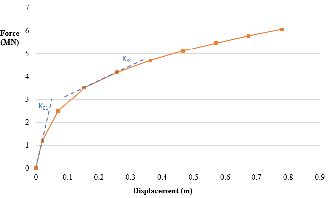
Non-linear foundations can be defined as a lookup table between the foundation node displacement and the reaction load from the foundation. These lookup tables are often referred to as “p-y curves” which refers to the lateral stiffness definition of a foundation, although lookup tables in all 6 nodal degrees of freedom can be defined. Non-linear curves result in a variable foundation stiffness (the p-y curve gradient), as illustrated in Figure 1.
Only a constant stiffness value can be included in the support structure stiffness matrix. Therefore, the initial slope of the curve (labelled \(K_{01}\) in the figure) is included in the support structure stiffness matrix, and the non-linear part is included as an applied load.
Dynamic model for non-linear foundations
For non-linear foundation p-y curves, support structure modal deflections are often not accurate enough to be used for looking up the foundation load in the p-y curve. This is because the non-linear nature of the p-y curve means that small differences in displacement can result in large differences in foundation stiffness. Consequently, the stiffness of the foundation and the reaction force may not be accurately predicted if modal displacements are used for the foundation load lookup. It is therefore desirable to use the finite element (FE) model displacements directly which more accurately determine the foundation deflections for lookup in the p-y curve.
The FE model displacements are found by solving: \(\bvector{f} = \bmatrix{K}\bvector{x}\), to find \(\bvector{x}\) for the support structure, where
\(\bvector{f}\) is the vector of applied loads = (external loads + inertial loads) on each node of the support structure,
\(\bmatrix{K}\) is the FE stiffness matrix for the support structure. This is constant.
\(\bvector{x}\) is the vector of support structure nodal displacements
The vector of FE displacements, \(\bvector{x}\), can then be used as lookup in the non-linear p-y curve.
Unfortunately, \(\bvector{f}\) is not known at the start of each time step, as it includes the effect of inertial forces, which depend on the system accelerations. Therefore, \(\bvector{x}\) isn’t known at the start of each time step either, so Bladed must use \(\bvector{x}\) from the previous time step when calculating the foundation applied loads.
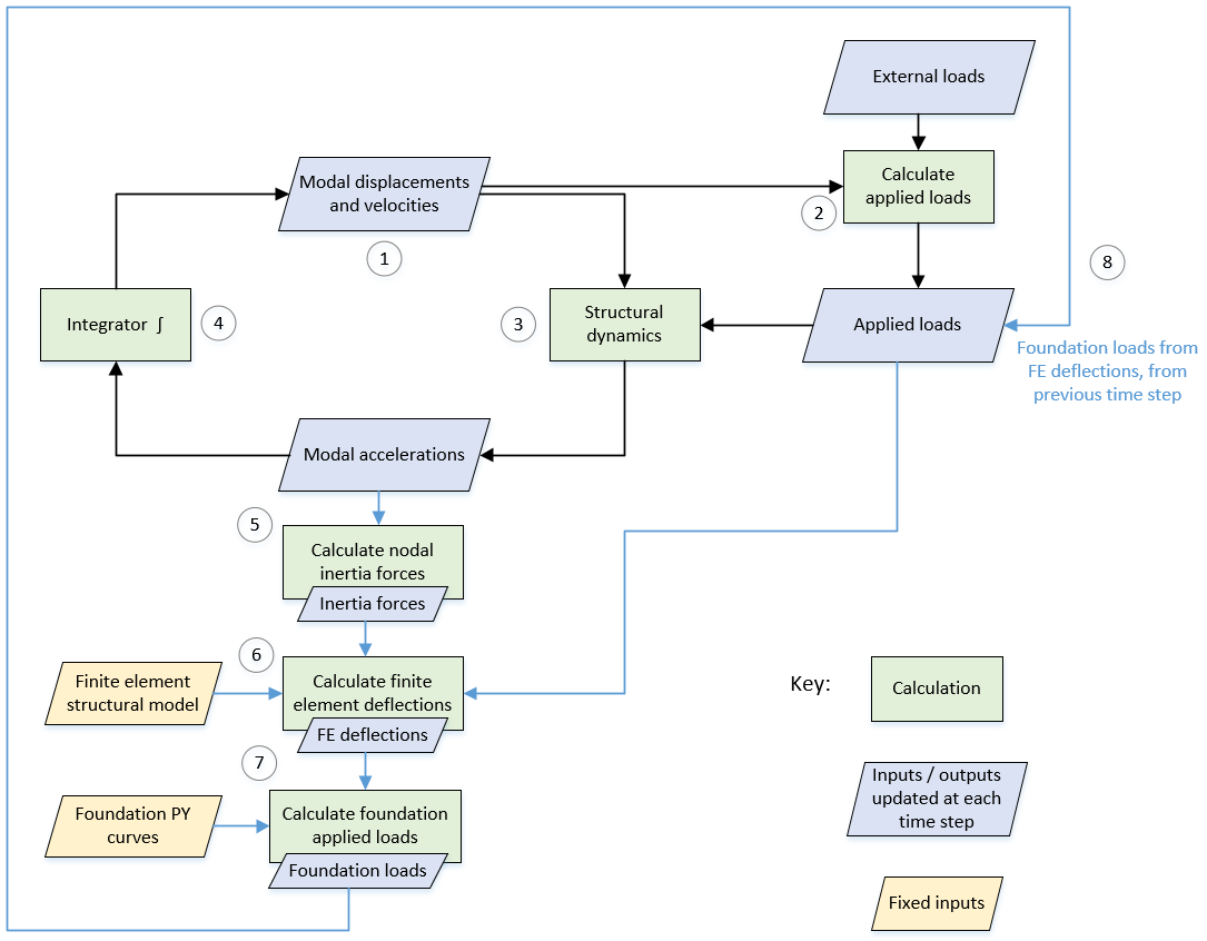
An algorithm schematic is presented in Figure 2 which shows the calculation carried out in Bladed when using the dynamic non-linear foundation load feature. The number of each step maps directly to the numbers in the flow diagrams depicted in Figure 2. Note that steps 1-4 are described in calculation procedure.
The modal accelerations are used to calculate the acceleration of each node, and therefore the inertial loading at each node can be calculated.
The equation \(\bvector{f} = \bmatrix{K}\bvector{x}\) is solved. The applied loads $\bvector\ $include contributions from inertia and external loading. \(\bmatrix{K}\) is the support structure stiffness matrix. The FE deflections \(\bvector{x}\) are found.
The FE deflections \(\bvector{x}\) are used to lookup the foundation forces in the p-y curves.
On the following time step, the foundation applied loads are used when evaluating the structural dynamics in step 3.
Last updated 30-08-2024