Dynamic Upwind Wake

The dynamic upwind wake uses a collection of models to describe the modification of wind conditions to the presence of a solitary upwind turbine. These include a wake model for computing the wake deficit dependent on the operating point of the upwind turbine. A wake meandering model that requires a low pass filtered wnd file to be generated. Please see "Bladed Project info options - O.pdf". And a model that simulates the increase in turbulence intensity due to the wake added turbulence.

This modelling option can be found in the Dynamic upwind wake screen under the menu options Specify > Wind....

Wake model

The initial wake profile is generated from the axial induction factors of the upstream turbine, such that the relative wind velocity is according to streamtube theory:

\[ \begin{equation} \bscalar{u_{r} = 1 - 2a_{r}} \end{equation} \]

Where \(\bscalar{a_{r}}\) is the axial induction factor at a given radius. In the near wake (considered as the first two diameters behind the rotor disc), the wake profile is stretched according to the following radial expansion, considering mass flow rate in the streamtube.

\[ \begin{equation} \bscalar{\int_{0}^{R_{w}}{r_{w}dr_{w}} = f_{w}\int_{0}^{R_{t}}{\frac{1 - a_{r}}{1 - 2a_{r}}r_{t}dr_{t}}} \end{equation} \]

Where \(\bscalar{r_{t}}\) and \(\bscalar{r_{w}}\) are the radial coordinates at the rotor disc and back of near wake respectively. \(\bscalar{f_{w}}\) is a calibration factor suggested by (Madsen et al, 2010) and is calculated from the mean axial induction factor at the rotor disc:

\[ \begin{equation} \bscalar{f_{w} = 1 - 0.45{\overline{a}}^{2}} \end{equation} \]

After the near-wake, the wake profile is then propagated according to the thin shear layer approximation of the Navier-Stokes equation:

\[ \begin{equation} \bscalar{{u\frac{\partial u}{\partial x} + v\frac{\partial u}{\partial r} = \frac{1}{r}\frac{\partial}{\partial r}\left( \varepsilon r\frac{\partial u}{\partial r} \right) }{= \varepsilon\left( \frac{1}{r}\frac{\partial u}{\partial r} + \frac{\partial^{2}u}{\partial r^{2}} \right)}} \end{equation} \]

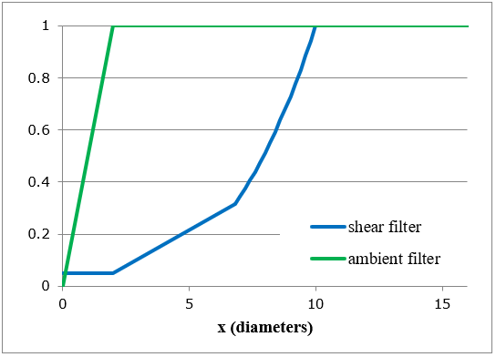
Where \(v\) is the radial component of the velocity and \(x\) is the distance downstream in the mean wind direction. The eddy viscosity, \(\bscalar{\varepsilon}\), is calculated by:

\[ \begin{equation} \begin{aligned} \bscalar{ &\varepsilon = \varepsilon_{shear} + \varepsilon_{ambient}, \\ &\varepsilon_{shear} = f_{shear}(x)K_{shear}B_{W}\left( 1 - u_{0} \right), \\ &\varepsilon_{ambient} = f_{ambient}(x)K_{ambient}I_{ambient}} \end{aligned} \end{equation} \]

\(\bscalar{B_{W}}\) (mixing length), \(\bscalar{K_{shear}}\) (shear calibration constant) and \(\bscalar{K_{ambient}}\) (ambient calibration constant) are user inputs. \(\bscalar{u_{0}}\) is the axial component of velocity at the centre of the wake, and \(\bscalar{I_{ambient}}\) is the ambient turbulence intensity. \(\bscalar{f_{shear}}\) and \(\bscalar{f_{ambient}}\) are filters as a function of distance downstream suggested by (Madsen et al, 2010). Their effect is to reduce the effective viscosity in the near wake and have been made by a calibration study.

Figure 1: Shear and ambient viscosity filters as suggested (Madsen et al, 2010)

Meandering wake

The wake meandering model is based on the assumption that the transport of the wakes in the atmospheric boundary layer can be modelled as passive tracers driven by the large-scale turbulence structures (see (Madsen et al, 2010)).

The meandering is modelled by tracking the positions of the centrelines of a cascade of wakes that are emitted from the upstream turbine at different time instances. These wakes travel through a turbulent wind field, that is low-pass filtered such that it only includes the large-scale turbulence structures. The lateral and vertical position of the wake centrelines will be stored once they have reached the downstream turbine. This will result in a pre-computed time history of the wake centre line position at the downstream turbine.

The meandering of the wake does not affect the wake deficit profile but determines a time-variant position of the wake centre-line. The lateral and vertical position of the centre-line, \(\bvector{y}\), is determined by the integral:

\[ \begin{equation} \bvector{y} = \int_{\bscalar{t_{0}}}^{\bscalar{t_{0} + \frac{\eta U_{ambient}}{X_{wake}}}}{\bvector{v}_{turb}(x,t)dt} \end{equation} \]

Where \(\bvector{v}_{turb}\) is the non-axial velocity vector due to turbulence (the axial component is not used), \(\bscalar{\eta U_{ambient}}\) is the longitudinal velocity of the wake (\(\bscalar{\eta}\) is a user input) and \(\bscalar{X_{wake}}\) is the downstream distance of the modelled turbine from the upstream turbine that generates the wake. Finally, \(\bscalar{t_0}\) is the time at which the wake is released. This initial time is used to compute an initial longitudinal position of the wake in the 3D wind field. Note that it is assumed that the upstream rotor position is always centred at hub height of the turbulent wind field as shown in Figure 2.

In vector notation \(\bvector{y}\) and \(\bvector{v}_{turb}\) can be written as below. Note that the definition of lateral and vertical direction is given in Figure 2.

\[ \begin{equation} \bvector{y =}\binom{\bvector{Y}}{\bvector{Z}} \end{equation} \]

\[ \begin{equation} \bvector{v}_{turb}\bvector{=}\binom{\bvector{v}}{\bvector{w}} \end{equation} \]

Figure 2: Definition of lateral, vertical and longitudinal directions in 3D wind field centred in the mid point of the wind field.

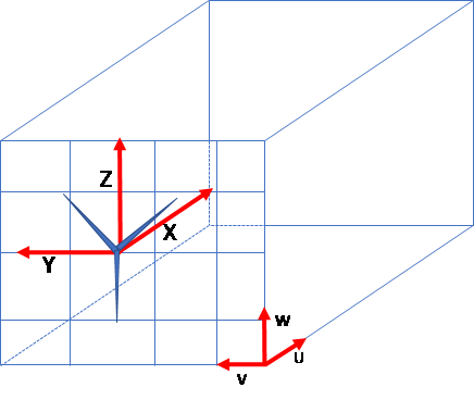
In case \(\bscalar{\eta = 1}\) the wake travels in longitudinal direction with the same speed as the ambient mean wind speed. This means that the wake will meander in the same turbulence "plane". In any other case the relative longitudinal location of the wake in the 3D wind field is computed as

\[ \begin{equation} \bscalar{X_{rel}} = \ \int_{\bscalar{t_{0}}}^{\bscalar{t_{0} + \ \frac{\eta U_{ambient}}{X_{wake}}}}{\bscalar{U_{ambient}(1 - \eta)}}dt \end{equation} \]

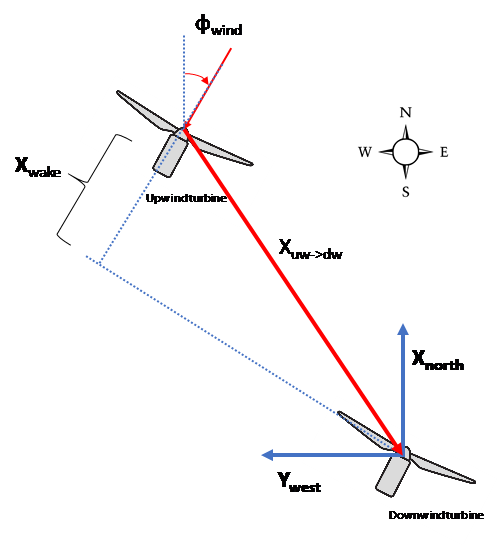
Note that the upstream turbine can be oriented at a distance North and West to the downwind turbine. The downstream travel (\(\bscalar{X_{wake}}\)) of the wake is then a function of the wind direction and the relative position of the upstream turbine. It is assumed that both the upwind and downwind turbine have no yaw misalignment relative to the wind, (see Figure 3).

The downstream distance can then be computed as follows:

The wind vector can be expressed in local West (\(\bscalar{Y_{west}}\)) and North (\(\bscalar{X_{north}}\)) coordinates.

\[ \begin{equation} \bvector{V =}\left| \bvector{V} \right|\binom{- \cos(\bscalar{\phi_{wind}})}{\sin(\bscalar{\phi_{wind}})} \end{equation} \]

The vector pointing from the upwind to the downwind turbine \(\bvector{(X_{uw \rightarrow dw})}\) is defined as:

\[ \begin{equation} \bvector{X}_{uw \rightarrow dw} = - \binom{\bscalar{X}_{north}}{\bscalar{Y}_{west}} \end{equation} \]

The downstream distance (\(\bscalar{X_{wake}}\)) is then computed by projecting \(\bvector{X_{uw \rightarrow dw}}\) into the direction of the wind vector

\[ \begin{equation} \bscalar{X_{wake}} = \frac{\bvector{X}_{uw \rightarrow dw} \cdot \bvector{V}}{\left| \bvector{V} \right|}=\bscalar{X_{north}}\cdot \cos\left( \bscalar{\phi_{wind}} \right) - \bscalar{Y_{west}}\cdot \sin\left( \bscalar{\phi_{wind}} \right) \end{equation} \]

Figure 3: Illustration of wake travel distance (\(\bscalar{X_{wake}}\)) as a function of location of upwind turbine and wind direction

Turbulence in the wake

If the eddy viscosity wake model is used, it is also possible to calculate the additional turbulence caused by the wake. The added turbulence is calculated using an empirical characterisation developed by (Quarton and Ainslie, 1990). This characterisation enables the added turbulence in the wake to be defined as a function of ambient turbulence \(\bscalar{I_{amb}}\), the turbine thrust coefficient \(\bscalar{C_t}\), the distance \(\bscalar{x}\) downstream from the rotor plane and the length of the near wake, \(x_n\). The characterisation was subsequently amended slightly by (Hassan, 1992) to improve the prediction, resulting in the following expression:

\[ \begin{equation} \bscalar{I_{add}=5.7{C_t}^{0.7}{I_{amb}}^{0.68}\left(x/x_n\right)^{-0.96}} \end{equation} \]

in which all turbulence intensities are expressed as percentages. Using the value of added turbulence and the incident ambient turbulence the turbulence intensity \(\bscalar{I_{tot}}\) at any turbine position in the wake can be calculated as

\[ \begin{equation} \bscalar{I_{tot}=\sqrt{{I_{amb}}^2+{I_{add}}^2}} \end{equation} \]

The near wake length \(\bscalar{x_n}\) is calculated according to (Vermeulen et al, 1981a) and (Vermeulen et al, 1981b) in terms of the rotor radius \(R\) and the thrust coefficient \(\bscalar{C_t}\) as

\[ \begin{equation} \bscalar{x_n=\frac{n r_0}{\left(\frac{dr}{dx}\right)}} \end{equation} \]

where

\(\bscalar{r_0=R\sqrt{\frac{m+1}{2}}}\)

\(\bscalar{m=\frac{1}{\sqrt{1-C_t}}}\)

\(\bscalar{n=\frac{\sqrt{0.214+0.144m}\left(1-\sqrt{0.134+0.124m}\right)}{\left(1-\sqrt{0.214+0.144m}\right)\sqrt{0.134+0.124m}}}\)

and \(\bscalar{\frac{dr}{dx}}\) is the wake growth rate:

\[ \begin{equation} \bscalar{\frac{dr}{dx}=\sqrt{\left(\frac{dr}{dx}\right)_\alpha^2+\left(\frac{dr}{dx}\right)_m^2+\left(\frac{dr}{dx}\right)_\lambda^2}} \end{equation} \]

where,

\(\bscalar{\left(\frac{dr}{dx}\right)_\alpha=2.5I_0+0.005}\) is the growth rate contribution due to ambient turbulence,

\(\bscalar{\left(\frac{dr}{dx}\right)_m=\frac{\left(1-m\right)\sqrt{1.49+m}}{\left(1+m\right)9.76}}\) is the contribution due to shear-generated turbulence,

\(\bscalar{\left(\frac{dr}{dx}\right)_\lambda=0.012 B\lambda}\) is the contribution due to mechanical turbulence, where \(B\) is the number of blades and \(\bscalar{\lambda}\) is the tip speed ratio.

Last updated 30-08-2024