Channel Combination

Use this calculation to combine and scale a number of signals. For example, this can be useful for generating a stress history for a particular point in the turbine structure, by expressing it as a linear combination of the various loads acting on the component. The stress history can then be used to calculate fatigue damage. The scale factors used for the linear combination should be such that the resulting signal is in the same stress units as are assumed in the fatigue damage calculation.

If Combine variables across different load cases is selected, it is possible to combine up to six signals from different calculations. Usually however, the signals to be combined will all come from the same calculation, so this option should be left unselected. This will give three options:

Channel Combination, which allows the choice of:

• an old Style of channel combination which allows channel combinations from Bladed versions 3.51 and older to be re-used (click Import details... and select whether to import the channel combination details, the list of load cases, or both), and

• a new style of channel combination (if neither check-box is selected) which provides much greater flexibility and ease of use.

Channel Tabulation, which allows a number of variables to be output to a single file.

Matrix Combination, which allows multiple outputs to be produced from multiple inputs through matrix multiplication.

In each case, first define the Combined Signal File No (from 1 to 260; up to 260 combined signal files may be generated for any load case), and enter a description for the file.

In the Tabulation case, there is a choice to keep the output files with the results of each original calculation, or to place them in a new location. If New directory is chosen, select a directory which will be used to replace any part of the file path which is common to all the runs which are to be processed.

Then click Channels and Load Cases to define the list of variables to be processed, and the list of runs for which the processing will be repeated. Each run should contain all the variables to be processed.

Multiple processing option

Channel combination

Select Variables, and click Add Variable to define the variables to be processed. Click Add Calculation to set up an equation for processing the variables. Any number of equations may be defined. Each equation will generate a new intermediate or output variable, which will be denoted #1, #2 etc. Each equation may process any of the input variables (which will be denoted $1, $2 etc.) together with any of the intermediate variables #1, #2 etc. Any of the intermediate variables which are given an output name will be output to the results file.

To edit an equation, highlight any part of it and use the editing options in the panel on the right. These can be used to enter specific values, such as input ($) or intermediate (#) variables or constants, to apply binary arithmetic or logical operators, or to apply unary operators. These include the conditional operator IF, and user-defined non-linear functions, which are entered as lookup tables – the calculation will use linear interpolation between table values, and for values beyond the end of the table the nearest point in the table is used.

To create a calculation that refers to its own previous value simply use the # value from the current equation. You do not need to use the prev() function here as the created variable already refers to its previous value when used in its own equation: So if you use “#1 + 1” in the equation of #1, this will add +1 to its previous value, which is initialised to zero at the start.

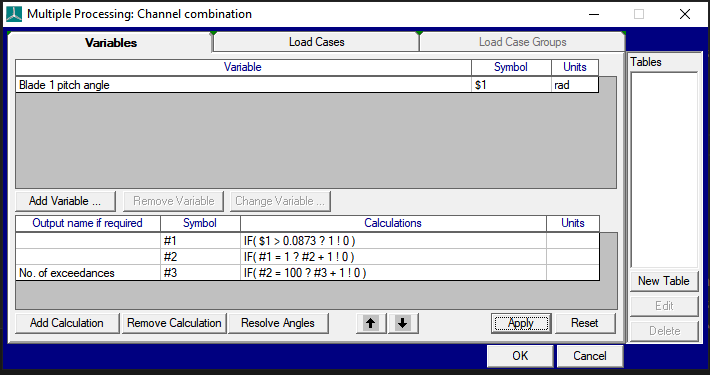
For example, in order to find out if and how many times a variable has been greater than a specified value for an uninterrupted period, you can setup a channel combination calculation as shown in Figure 1.

In this example, we are calculating how many times the pitch angle exceeds 5 deg (0.0873rad) for an uninterrupted 5 sec (100 time steps).

Figure 1: Multiple processing: Channel combination

Use Resolve Angles to generate a whole set of equations representing the resultant of two orthogonal loads resolved into different angles. Select the 0 \(\bunit{deg}\) and 90 \(\bunit{deg}\) loads from the list on the right of the screen – for example, the hub My and Mz loads could be selected. Then define a range of angles to resolve over, and provide a name for the output variables if they are to be output. If the 0 \(\bunit{deg}\) and 90 \(\bunit{deg}\) loads are \(V_{\text{0}}\) and \(V_{\text{90}}\), then for each angle θ an equation is created which generates \(V_{\text{0}} \cos \theta + V_{\text{90}} \sin \theta\). The output name for each variable (if specified) will automatically have the appropriate angle appended.

Finally click Load Cases to set up a list of load cases for which the resulting set of channel combinations will be repeated.

Tabulation

Select Variables to define the list of variables to be tabulated. For each variable, select the desired units to be used for the tabulation.

Finally click Load Cases to set up a list of load cases for which the resulting set of channel combinations will be repeated.

When the calculation is run, the output may be chosen to be in ASCII or binary format. Selecting ASCII format will tabulate the selected variables as columns in a tab-delimited text file, with column headings describing each variable.

Matrix combination

The matrix combination calculation is available for example to set up an influence matrix, by defining a set of output loads as a linear combination of a set of input loads.

Select Variables, and click Add Variable to define the variables to be processed. Click Add Matrix to set up a matrix for processing the variables. Click Add Output to specify the outputs from the matrix combination. Any number of matrices may be defined. The size of the matrix is determined by the number of input variables and the number of outputs.

To edit a matrix, either type directly into the matrix grid or copy and paste into this grid.

Finally click Load Cases to set up a list of load cases for which the resulting set of matrix combinations will be repeated.

Once a matrix combination has been set up, the Vector Combination option becomes available. This allows outputs from a matrix combination to be processed further as a vector. Click Define details to set up the vector combination.

The vector combination is set up in a similar way to the channel combination. Each equation may process the vector of outputs from each matrix (denoted M1, M2 etc) to produce a further vector of outputs (denoted V1, V2 etc). Click Add Variable to defined additional variables which may also be used in the equation if required.

Old Style channel combination

Select Variables and click New to define a new output signal, and enter a description for it. Select one of the available units for the signal if appropriate.

For each output variable, click Add Variable… to select the required input variables. Specify any factor, offset and other unary operators to be applied to each input signal before it is combined with the other input signals. The Factor is applied first, then the Offset, then any Unary operators are applied. If several unary operators are specified, they must be separated by | (a vertical bar). They will be applied in order, starting from the right-most. Allowed operators are:

• SIN: sine (of a value in radians)
• COS cosine (of a value in radians)
• ABS: absolute value
• SQRT: square root
• INV: reciprocal
• +n: Add a number n
• -n: Subtract n
• $\times$n: Multiply by n
• /n: Divide by n
• ^n: Raise to the power n

where \(n\) is a real number, which may be negative. For example, `SIN|x-3.2|^-0.2|ABS|+0.1 would calculate \(\sin(-3.2(|*x*+0.1|^{-0.2}))\) from the input signal \(x\).

Then select how the resulting input signals are to be combined. This may be by

• addition,
• squaring and adding, then taking the square root of the result, or
• multiplying.

Finally click Load Cases to set up a list of load cases for which the resulting set of channel combinations will be repeated.

Single channel combinations

From Channel combination and Tabulation, select Combine variables across different load cases to generate a new variable not attached to any existing load case. You will then be asked for a directory and run name for the output when you start the run. In this case, click the numbered channel selection buttons to define up to six signals to be combined. The signals may be from different runs or load cases if desired. For each signal, enter a scale factor and an offset. Enter a description for the combined signal, and choose units if appropriate.

The scale factors \(a_i\) are applied before the offsets \(b_i\). The result of the calculation can be expressed as:

\[ \begin{equation} y = \Sigma (a_i x_i + b_i) \end{equation} \]

if Simple Addition is selected. If Square-Add-Square Root is selected, the result is

\[ \begin{equation} y = \sqrt{\Sigma (a_i x_i + b_i)^2} \end{equation} \]

Enter a description for the combined signal, and select one of the available units for the combined signal if appropriate.

Last updated 10-09-2024