Methodology

This article describes the methodology employed to assess the quality of the turbulent wind data generated using Bladed. The basic principle of the verification approach is by comparing the statistical properties of the turbulent wind time series against the theoretical quantities in terms of spectra and coherence. The general settings used for generating the turbulent wind field and the data processing method are further described in the subsequent sections.

Wind File Setup

For each verification study for a particular case, a turbulent flow field is generated with the specifications listed in Table 1. These parameters are generally constants throughout the analyses, unless stated otherwise for each turbulence model of interest. The calculations are carried out for sufficiently large domain in all three directions (note that the longitudinal domain also refers to temporal domain).

Table 1: General parameters to define the turbulent wind field in the verification studies.

Parameter	Value
Longitudinal domain size	24,000 m
Lateral domain size	210 m
Vertical domain size	210 m
Mean wind speed	10 m/s
Duration of the simulation	2,400 s
Sampling frequency	13.6 Hz
Lateral grid number	51
Vertical grid number	51 or 26
Velocity components investigated	\(u\), \(v\) and \(w\)

Data Processing

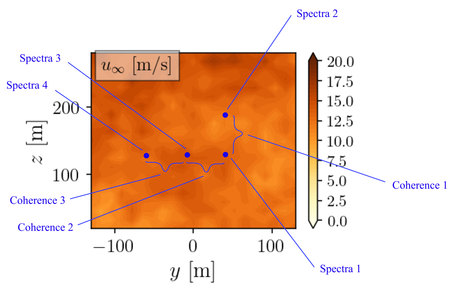
For each generated turbulent field data, a post-processing analysis is done to recompute the spectra and coherence associated with the wind time series. Figure 1 illustrates the grid points being used for sampling the time series data to compute the spectra and coherence. The spectra can be computed based on the individual grid points while the coherence calculations require time series data sampled from two grid points. It is to be noted that in order to simplify the present evaluations, the coherence is only sampled at grid points separated strictly laterally or vertically, i.e., no diagonal separation distance is considered.

For each grid point plotted in Figure 1, the turbulent wind time series will fluctuate according to a specific spectral model depending on the turbulence model being adopted. In theory, the spectra for each data point will be exactly the same if the turbulent field is computed for extremely long period of time at a small sampling time (high sampling frequency). This is impractical in real application, hence there will be some slight discrepancies between the spectra obtained at one point compared to the other points.

Figure 1: Illustration of the grid points to sample the turbulent wind time series used for calculating the spectra and coherence. The sampling process is done strictly in lateral and vertical dimensions. Dots represent the corresponding grid point being evaluated.

The similarity of the time series from one data point to the other data point is represented by coherence. This is measured as the ratio of the cross-spectra (\(S_{ij}\)) to the auto-spectra (\(S_{ii}\) or \(S_{jj}\)) at each data point, defined as:

\[ \begin{equation} \gamma^2 (f,r) = \dfrac{|S_{ij}(f)|^2}{S_{ii}(f) \ S_{jj}(f)}, \end{equation} \]

with \(f\) defining the frequency, \(r\) the separation distance between two grid points being evaluated (not necessarily the adjacent grid point) and \(i\) as well as \(j\) being the grid point of interest. In theory, for the same value of \(r\), coherence function should be the same regardless of the position of the grid points. This is true as long as the turbulent field is computed for extremely long period of time at a small sampling time, which is not practical.

In the present investigations, spatial (ensemble) averaging is performed for both spectra and coherence functions. For the turbulent wind spectra, this is simply done for all grid points. However, for the coherence, this is done depending on the separation distance. For example, when coherence is evaluated at a separation distance \(r\) equal to the distance between the adjacent grid points (separation distance is equal to 1 grid step), it will have more data points for averaging than a case where the separation distance is set to 2 or 3 grid steps. Mathematically, the averaging process for the spectra and coherence are formulated as:

\[ \begin{equation} S (f) = \dfrac{1}{N}\sum^{n=N}_{n=1}{S_{ii,n}(f)} \end{equation} \]

\[ \begin{equation} \gamma^2 (f,r) = \left[\dfrac{1}{N}\sum^{n=N}_{n=1}{\gamma_n(f,r)}\right]^2, \end{equation} \]

with \(n\) being the data sampling which ranges from 1 to the maximum sampling number \(N\).

Last updated 17-07-2024