CFD.ML wake & blockage model
CFD.ML is a machine-learning based, surrogate model for DNV's state-of-the-art, high-fidelity CFD RANS model of wind farm flows.
In contrast to the engineering wake & blockage models, CFD.ML aims to capture the entirety of turbine aerodynamic interactions (wake & blockage together), and is not tuned to any particular SCADA dataset. It approximates RANS CFD - a method derived from first principles. The model is trained to predict only the pair-wise aerodynamic impacts of turbines on each other - CFD.ML does not contain any analytic formula for wake or blockage propagation. It is the Navier-Stokes equations underlying the RANS CFD model, together with assumptions regarding atmospheric boundary layer height, stratification and the simplified actuator-disc model for the wind turbines that result in particular wake & blockage propagation patterns, which are then encoded by the machine learning part of CFD.ML.
CFD.ML is based on years of DNV research and has primarily been developed to interpolate between the computationally intense RANS CFD simulations - effectively increasing their directional resolution at a fraction of time otherwise needed to perform CFD for every directional flowcase. The significant operational experience gathered in that context, enabled the roll-out of CFD.ML as a stand-alone wake & blockage model in WindFarmer. As further model improvements are planned in the near future, CFD.ML is at the moment released in beta.
The original method is described in detail in [38]. The application of CFD.ML as a stand-alone model in energy production assessment of wind farms has been postulated publically during WindEurope Technology Workshop in 2023. These topics were also discussed in DNV's webinar:
At the heart of CFD.ML is a graph neural network (GNN) - a variant of neural networks well suited for learning physical interactions between objects. The GNN is trained on a large batch of real life CFD RANS simulations to predict the turbine interactions in a wind farm array.
Once a trained GNN is available, the process of estimating turbine interactions with CFD.ML has three main steps:
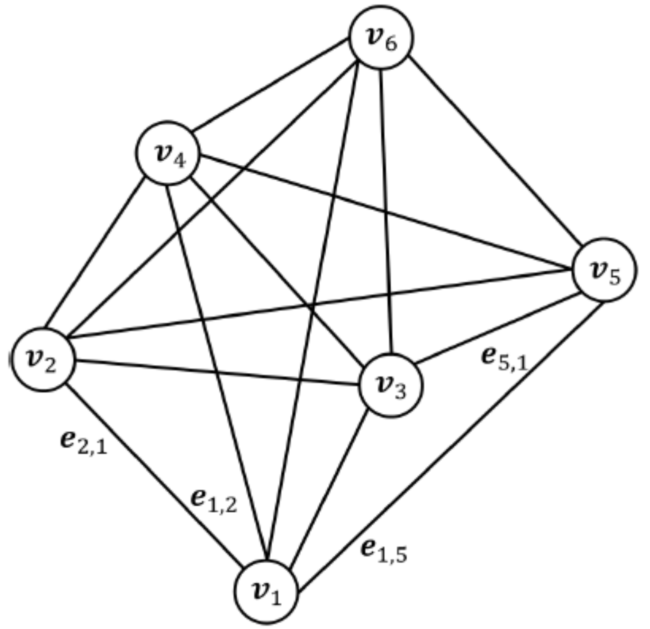
- [Step 1] with each turbine being a vertex of a graph, $ v_{i} $, and each turbine interaction between a turbine pair assigned to an edge, $ e_{i,j} $, with i denoting the receiver turbine, and j denoting the (wake and/or blockage) sender turbine.
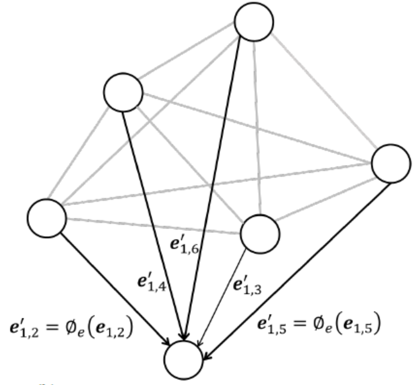
- [Step 2] the network approximates turbine interactions in a pair-wise manner, independently for each pair. This is done inside function $ \phi_{e} $, which takes the properties of the corresponding edge $ e_{i,j} $ as inputs and returns the aerodynamic impact of the sender on the receiver turbine. The edge properties are: downwind and crosswind separations between turbines, the sender turbine geometry and its thrust. $ \phi_{e} $ encodes the turbine interaction patterns learned from CFD simulations and is shared across the graph.
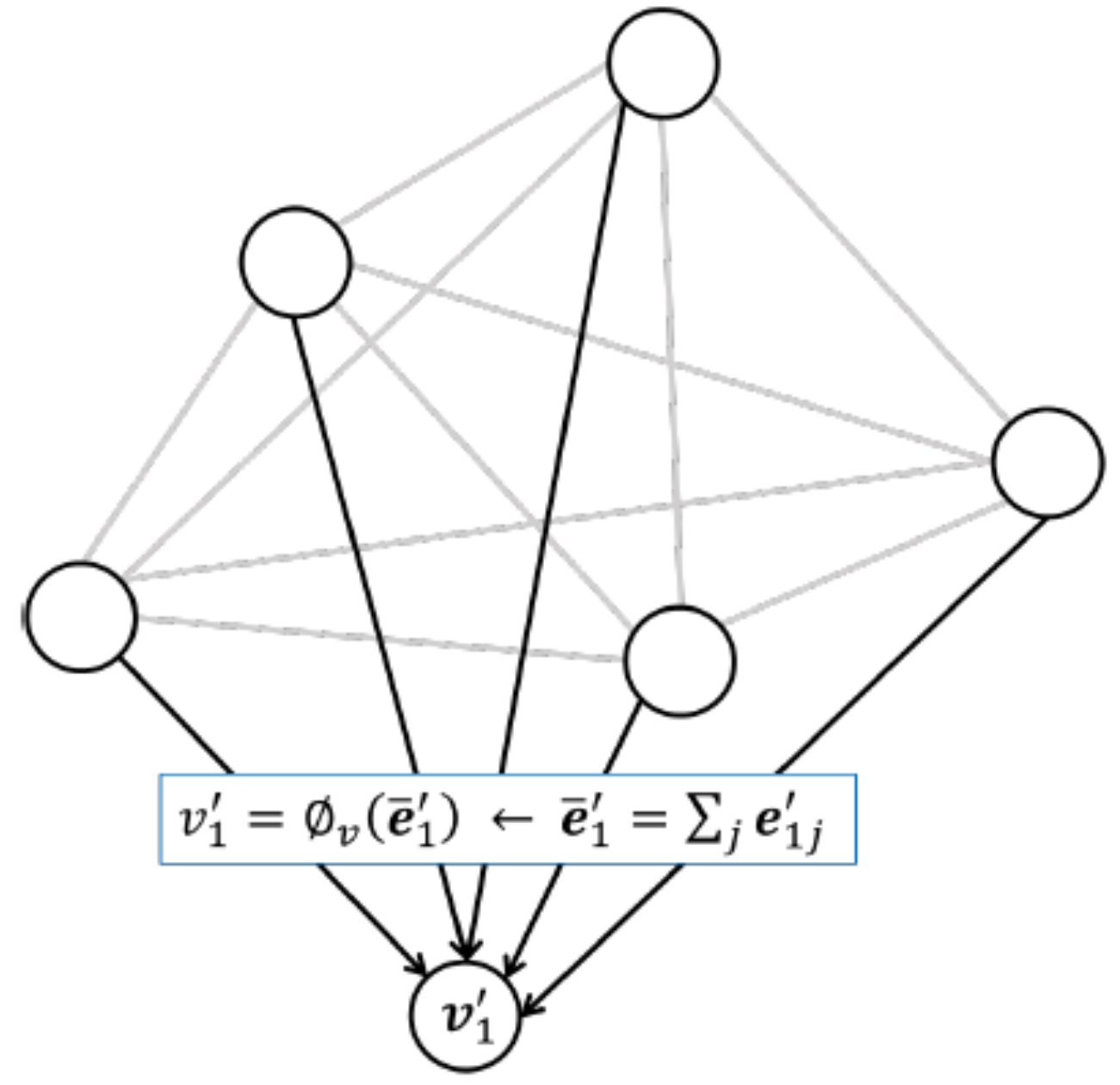
- [Step 3] the interactions coming from all the neighbours of turbine i are aggregated by the function $ \phi_{v} $ to produce the overall, combined turbine interaction effect experienced by turbine i, expressed as a ratio of the actual incident wind speed at that turbine, to the incident wind speed it would have experienced had it operated in isolation. In the current implementation the aggregation function is simply the sum of all the partial impacts.
| Step 1 | Step 2 | Step 3 |
|---|---|---|
 |
 |
 |
Using CFD.ML to estimate a blockage correction
The wind speed deficits (or speed-ups) predicted by CFD.ML contain the coupled impacts of both wakes and blockage. However, a post-processing step may be performed in addition to the core calculation to isolate a CFD.ML blockage correction. The CFD.ML blockage correction is an alternative to the blockage correction from the BEET model. The energy-based blockage correction can be applied to engineering wake models which do not account for upstream and lateral flow phenomena. The advantage of CFD.ML over the BEET is that the blockage-related wind field perturbations are captured on a per-turbine basis, as opposed to farm-average correction. Also, the CFD model settings that underlie CFD.ML's training set have been updated relative to what BEET was trained on.
How well does CFD.ML reproduce RANS CFD?
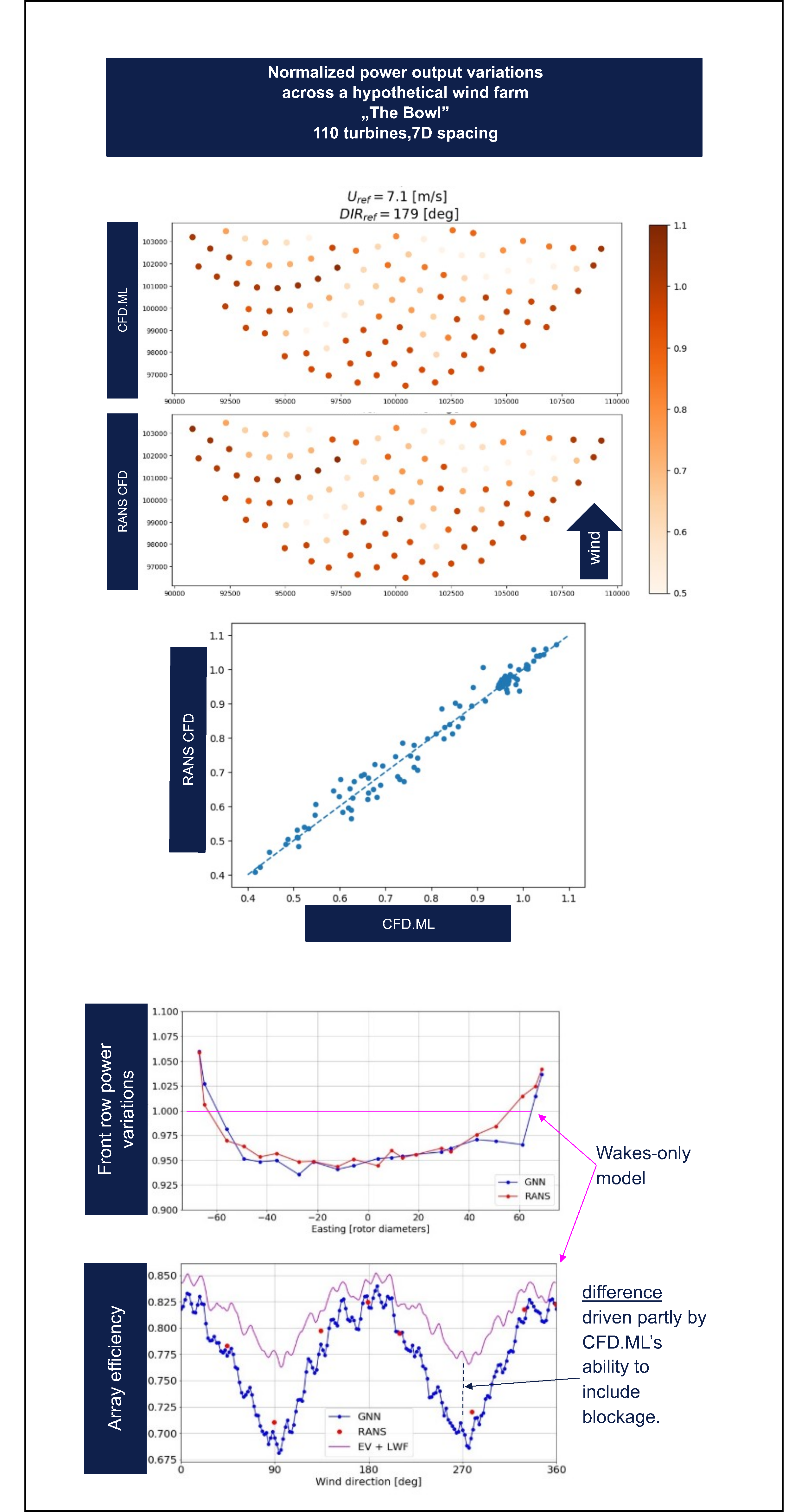
CFD.ML's skill at replicating RANS CFD is demonstrated below, on a hypothetical wind farm case. Despite the relatively complex array geometry, the per-turbine patterns of normalized power outputs are well captured by CFD.ML inside the array (where they are wake-dominated), as well as along the front, southern row of the farm (where the variations are blockage-dominated). The overall wind farm efficiency as function of wind direction is also matching reasonably well.
Usage
Whilst in beta, CFD.ML is made available only through WindFarmer Services API.
This requires the user to make the call using tools like Postman, a Python script or another language of choice. In both cases it is convenient to generate the json inputs for an annual energy production calculation using WindFarmer: Analyst's Automation module.
Examples of how to request an annual energy production with CFD.ML wake modelling using WindFarmer: Analyst's scripting and Python are published in the automation examples repository.
In the near future, direct calls to the WindFarmer Services API from within WindFarmer: Analyst will be possible.
Limitations of the beta version
Whilst in beta, the CFD.ML API rejects requests which would take too long to compute (>15min). The resulting turbine count limit depends an a combination of settings such as: directional resolution, number of wind speed bins to simulate, inclusion of efficiency variants etc. With typical settings it is currently only possible to calculate AEP for farms not larger than 180 turbines.
In the near future, upgrades to the cloud infrastructure running CFD.ML are planned, which should significantly raise these limits.
The training set
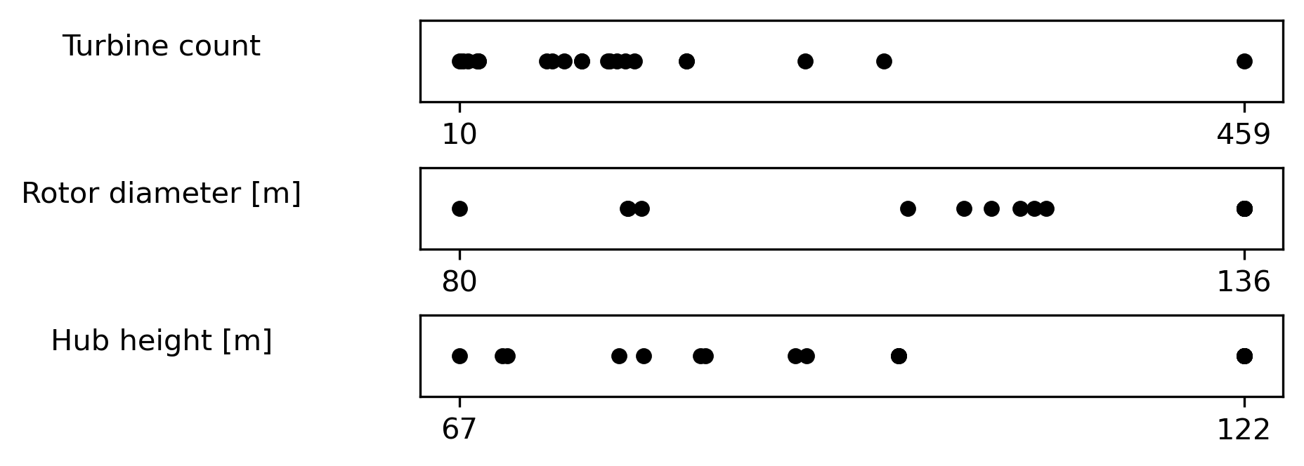
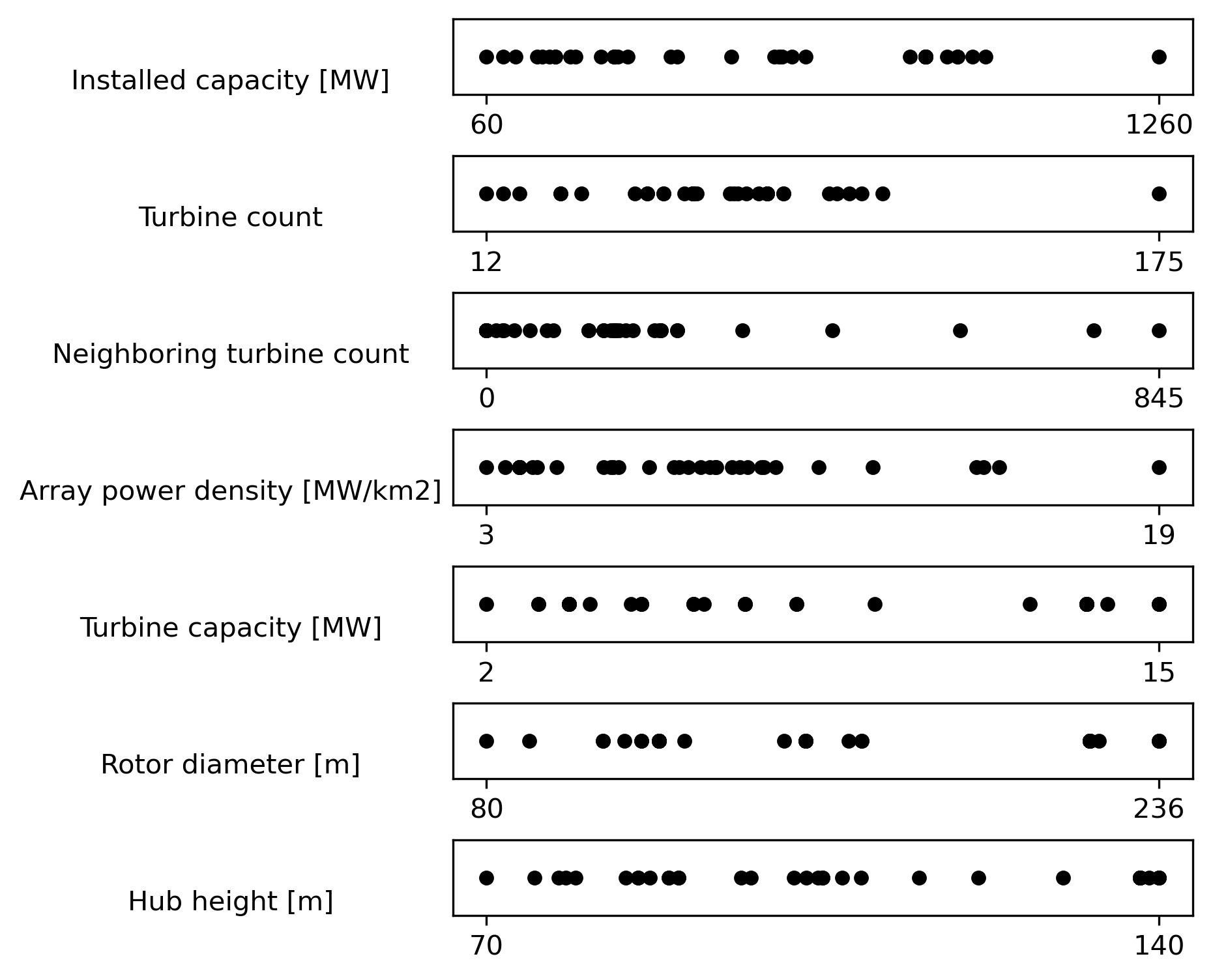
One should be mindful of not to apply CFD.ML outside of the training envelope of the model. The characteristics of the different wind farm CFD simulations used to train the latest onshore and offshore GNNs are presented in the figures below to demonstrate the envelope of the model training.
Due to the significant differences in characteristics of offshore & onshore boundary layers, separate GNNs are trained for each case to improve the accuracy of predictions. Currently, those GNNs are trained on a set of CFD simulations with conventionally neutral atmospheric boundary layer. However, in the near future DNV plans to improve the method such, that CFD.ML may account for atmospheric stability and boundary layer height.
The set is continuously updated as more farms get simulated or modelling upgrades are rolled out. Users are advised to use the most recent GNN. To allow reproducibility and traceability of historical results (for example in the context of minor updates to the energy production assessments), the older versions of the GNN can also be selected for calculations.
Please also note, that the onshore GNN has been trained on wind farm simulations in predominantly flat terrain.
