Large Wind Farm Correction | WindFarmer Documentation

Correction for large wind farms

The modelling of wind farms is traditionally a two-step process. In the first step the ambient wind flow without the presence of a wind farm is established. The wind turbines are placed within this wind flow in the second step. The ambient wind flow is assumed to be independent from the wakes generated by the wind turbines.

It is well-recognised that wind turbines do not only react passively to the wind regime, but at the same time they are part of it [15], [16], [17], [18]. Qualitatively, the wind farm can be thought of an area of higher roughness. The boundary layer profile local to the wind farm is disturbed by the extraction of momentum by the wind turbines. In particular, offshore wind farms cause a more pronounced local effect similar to an onshore forest, due to the lower roughness offshore. Onshore the effect of a large wind farm is less pronounced and to some degree masked by the higher roughness of the local terrain.

A large wind farm correction was developed by Garrad Hassan [19] and [20], based on modelling the disturbance caused by each individual turbine. This allows numerous wind farm layouts to be considered during the design phase of a wind farm layout. The model approach can be described in three steps:

Use the wind flow model and data of choice that best describe the ambient wind flow over the proposed wind farm site.
Place the turbines in the wind flow and calculate the large wind farm correction to the ambient flow due to the presence of the turbines.
Use a standard wake model with the corrected ambient wind speeds as boundary conditions to describe the inter-turbine wake deficits.

The second step above details an empirical correction to describe the disturbance of the atmospheric flow caused by the wind farm. This breaks with the traditional assumption that the wind flow can be treated as independent from the wind farm. The large wind farm correction consists of the following components:

Boundary layer modification – establishes the magnitude of correction to the ambient wind profile downwind of each individual turbine
Wind turbine density – considers relative turbine positions and decides if a correction should be applied in a particular direction sector
Row-to-row distance – the correction is applied only if adjacent lines of turbines are closer than a threshold
Downstream recovery – from a certain distance downstream, the wind speed recovers to ambient levels and no correction is applied.

The component models are presented in the following sections.

Boundary layer modification

Momentum is continuously generated on top of the boundary layer and is transferred downward to the ground surface in a dynamic equilibrium. Wind turbines that take out some of this momentum are part of the dynamic equilibrium similar to trees or other roughness elements. However as the impact of the wind turbines on the boundary layer profile is not yet well researched, we take some guidance from forest canopy and roughness change models.

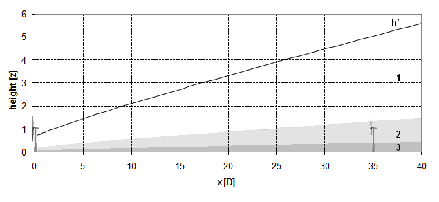
Internal boundary layer (IBL) development after disturbance caused by the first turbine, with Zones 1, 2 and 3 marked. The ambient wind speed for the downstream turbines is reduced.

An internal boundary layer (IBL) develops from each turbine location. The height (h) of the IBL for a roughness change, as a function of the fetch (x) and (z’₀), the larger of the two roughness values (z₀₁) and (z₀₂), can be determined from

$$\frac{h}{z_{0}^{'}}\left( \ln\frac{h}{z_{0}^{'}} - 1 \right) = 0.9\frac{x}{z_{0}^{'}}$$

To take into account that the momentum is not extracted at ground level, an offset of 2/3 hub height (z) is used leading to a new height (h’). The disturbance to the ambient wind speed (u₁) is injected in the flow over an area with the dimension of the upstream turbine rotor. This spatial dependency is considered in the model by introducing a vertical offset to z resulting in a new height z’. The wind speed (u) is then expressed as:

In the upper part of the IBL (Zone 1) the free wind speed is unchanged compared to the upstream conditions. In the lower part (Zone 3) the free wind speed changes according to roughness length z₀₂ and the downwind distance from the roughness change. In Zone 2 the free wind speed is interpolated between the lower and the upper section.

The resulting free wind speed is shown below for a turbine downstream of another turbine of the same hub height and rotor diameter, where the large wind farm criteria apply.

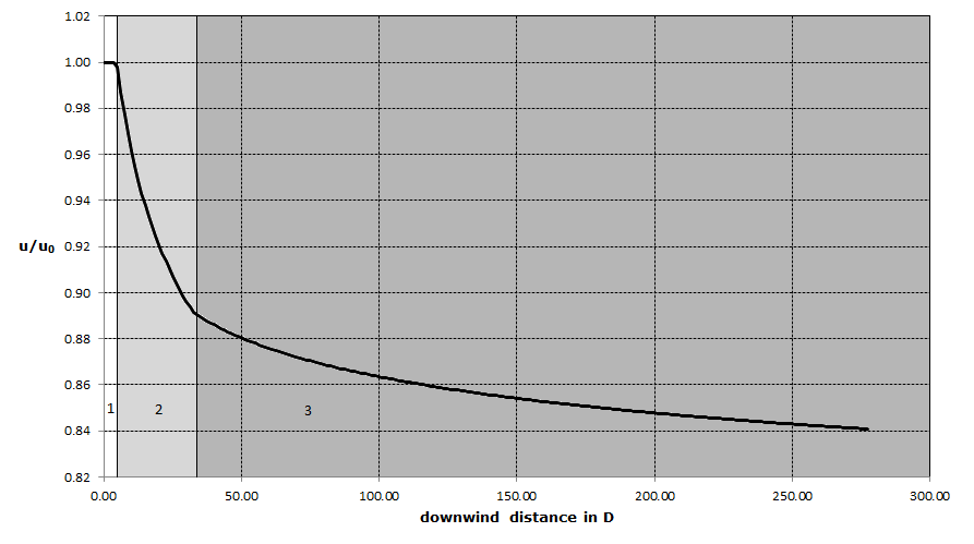
Reduced free wind speed for a turbine downwind of a turbine causing the large wind farm effect. The shading marks the zone of the IBL where the lower blade tip of the downstream turbine is located.

Wind Turbine Density

The momentum extracted per given area increases with the number of wind turbines in that area. Changing the area roughness to achieve this is an option, but it is impractical for wind farm design purposes, as the distribution of wind turbines may be irregular and is subject to iterative change and no fixed relationship with roughness can be established. Instead, a geometric measure of turbine density is used.

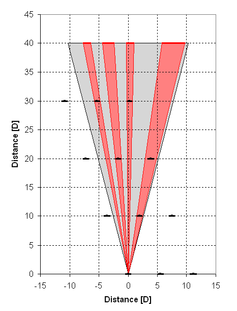
A geometric model is used to consider the turbine density for a 30 degree sector. The large wind farm correction to ambient wind speed is applied for wind arriving from the red sectors.

For each small direction sector, the horizon is scanned from the target turbine and the presence of upstream turbines is detected. The ambient wind speed correction is applied if and only if one or more turbines are present in the sector.

The consequences of the geometric model are that the overall magnitude of the correction is reduced with distance from turbines due to a smaller aspect ratio; and increased at a fixed distance with increased turbine density due to more turbines contributing.

The geometric model considers how much of the horizon is filled with turbines. Wake expansion is not considered in this step, since the model is to be used in conjunction with standard wake models that already consider the effect of wake expansion and consequential wake recovery.

Wind blows along wind farm geometry axis

When the wind direction is such that it blows along the turbine rows, and the cross-wind spacing between the rows is more than a given number of turbine diameters, then the wind turbine wakes in each row are considered to develop independently of other rows. Experimental evidence suggests that no large wind farm correction should be applied for this narrow wind direction sector.

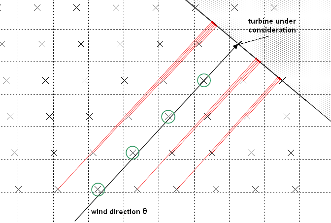
The crosswind distance is determined by projecting upstream turbines onto a plane perpendicular to the flow direction.

Downstream recovery

The disturbance of the wind profile caused by a wind turbine is expected to subside after a certain distance. Investigation is ongoing to establish details of the processes and relevant scales. However, as an initial approximation, this recovery can be modelled as exponential.

The recovery is calculated using

$$u_{r} = u_{1}\left( 1 - \left( 1 - \frac{u}{u_{1}} \right)*0.5^{\frac{x - x_{\textrm{start}}}{x_{50\%}}} \right)$$

where

x_start start distance for the recovery function

x_50% distance from the start distance, where the large wind farm wind speed correction has reduced to 50%

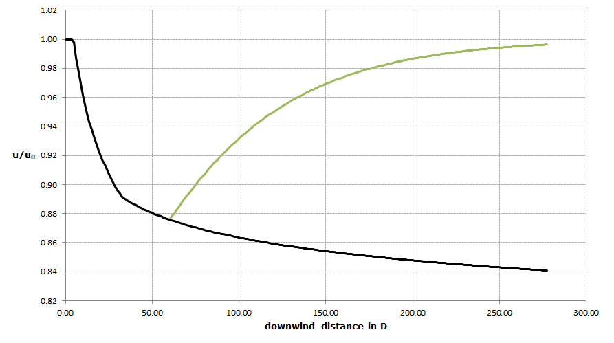
Reduced ambient wind speed (black line) with exponential recovery to ambient level (green line).

Model application

For every direction step the model checks if there are upstream turbines causing a wake.
If this is the case, the distance to the neighbouring rows is checked.
If the row distance is less than the maximum row spacing value where wakes develop independently from the neighbouring rows, then the correction of the free wind speed is applied.
For all upstream turbines the free wind speed is reduced with downwind distance up to the distance of the individual downwind turbines.
The resulting free wind speed with the large wind from correction at the downwind target turbine is the lowest free wind speed caused by one of the upstream turbines.
The wake effect is then calculated in the usual manner, using the large wind farm corrected free wind speed at the individual downwind turbines.

Model parameters

The parameters you need to edit in the calculation are

Parameter	description
Base roughness	Represents the surface without wind turbines. For onshore applications, a single value of Base roughness, representative of the site and surrounding area is appropriate. For offshore sites a value for the Base roughness of 0.0002 m is appropriate.
Increased roughness	Represents the effect of the wind turbines. An increase from the Base roughness between 0.02 and 0.03 m has been found to provide a good match. A higher value of 0.05 m can be used, when looking at specific wind speed cases with deep wakes. The default setting for the increased roughness is 0.06 m.

If you have WasP available, you may calculate base roughness via scripting.

Advanced parameters:

Parameter	description
Geometric width	determines the sector for which an upstream turbine has an affect on the downwind turbines. The default setting is 1 turbine diameter.
Maximum row spacing	Used to detect situations when the wind blows along a row of turbines, when the offshore deep array effect is not visible in the wind farm data. The row spacing represents the distance to the next row of turbines in the projection plane perpendicular to the wind direction. If this distance is greater than the maximum row spacing, the correction is not applied. The default value is 5 turbine diameters.
Start and 50% deficit distance parameters for recovery.	It is expected that the total disturbance declines as the distance behind the wind turbine increases. An exponential recovery to the unaffected free stream conditions is assumed behind the recovery start distance. DNV apply 120 and 40 rotor diameters for the start and 50% recovery settings respectively for offshore projects.