wind analysis
Monthly stats GenerateStats, ExportStats
ExportStats efficiently creates data coverage summaries, report tables, long-term mean wind speed and general statistics. ExportStats allows monthly temperature, pressure and any other measurement to be reported for any number of sensors in one output.
How each signal type is handled is summarised below:
Mean – Reports the mean of the time series
Min – Reports the min of the time series
Max – Reports the max of the time series
Stdev – Not supported.
Monthly summary
| Month | M2~A46~Mean | Coverage (Months) | |
|---|---|---|---|
| Jan | 10.004 | 2 | 2 months = two months with 100% coverage going into January wind speed of 10 m/s |
| Feb | 10.840 | 1.91 | |
| Mar | 10.923 | 1 | |
| Apr | 9.756 | 1 | |
| May | 9.747 | 1 | |
| Jun | 10.869 | 1 | |
| Jul | 11.770 | 1 | |
| Aug | 12.176 | 1 | |
| Sep | 11.635 | 1 | |
| Oct | 9.736 | 1.76 | |
| Nov | 9.801 | 2 | |
| Dec | 9.509 | 2 | |
| Annual | 10.562 | 16.66 | Annual value is the mean of monthly means and coverage of 16.66 months = period of valid data (1.4 years) |
Note – The monthly summary table always reports the average of the individual months, for example if the function is used on windspeed~Max for January the average(Max of each January) will be reported.
Additional statistics
ExportStats also includes summary statistics of the input time series.
| Overall | mDB1~T8~Mean | |
|---|---|---|
| Min | -7.766 | Minimum value in the input time series |
| Max | 24.370 | Maximum value in the input time series |
| Mean | 7.222 | Mean of the input time series |
| Valid Data (Years) | 5.182 | Years of valid data |
| Period (Years) | 5.475 | Years of measurement from start to end of valid data |
The period of data in years is defined by on first and last timestamp of the load data in the WindApp project for time series variables. This improves the estimation of the period when there is invalid data at the start and end of the data loaded into the WindApp project.
This becomes time between the first and last timestamp of valid data for calculated time series.
Monthly Statistics respects regional settings
The data format in the monthly stats output file respects the regional setting on your computer. This allows the output file to be used in excel with the correct date formatting automatically.
Turbulence intensity distributions
Turbulence intensity is calculated as Standard deviation of windspeed / Mean windspeed
If there are fewer than 10 records in any one wind speed and direction bin then the a + is printed in the word report generated by CreateTurbulenceIntensityDistribution. For calculations, if there are fewer than 10 records in any one bin then the all directional mean turbulence intensity is used. (E.g. in a wti file exported from ExportWTI or stored in the workbook).
The all directional turbulence intensity is calculated by taking the mean of all the time series turbulence intensity values above the low wind speed cut off.
Correlations
Linear correlation methods are used to derive speed trends between reference and site wind speed measurements. It is assumed that for each direction sector the pairs of wind speed data can be fitted to a straight line that is characterised by its slope and offset. To calculate slope and offset, either a least squares method or a PCA method can be used.
The general linear relationship between site and reference wind speed is therefore defined as
$$y = a + b \cdot x$$
where x is the wind speed at the reference station, b is the slope and a is the offset of the linear fit, and y is the concurrent wind speed at the site.
The correlation coefficient indicates the strength and direction of a linear relationship between two random variables. It ranges from +1 to -1. A correlation coefficient of +1 means that there is a perfect positive linear relationship between the variables: when the reference variable increases, the dependent variable also increases. A correlation coefficient of -1 means that there is a perfect negative linear relationship between the variables: when the reference variable increases, the dependent variable decreases. A correlation of 0 means that there is no linear relationship between the two variables.
The linear correlation coefficient is defined as
$$r = \frac{\sum_{i}^{}{\left( x_{i} - \bar{x} \right)\left( y_{i} - \bar{y} \right)}}{\sqrt{\sum_{i}^{}\left( x_{i} - \bar{x} \right)^{2}\sum_{i}^{}\left( y_{i} - \bar{y} \right)^{2}}}$$
Least Squares method
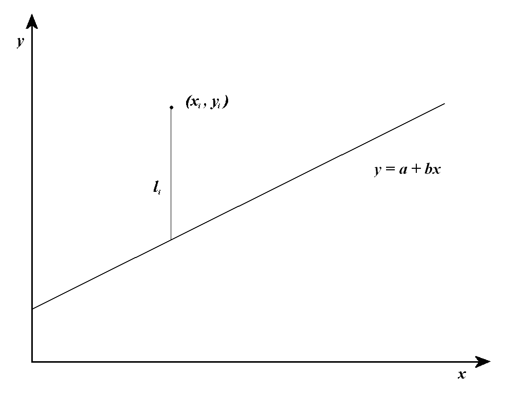
Assume that the measured wind speed is xi at the reference station and yi at the site, at a specific time. For a number n of such points, the least square method derives the linear fit that minimises the sum of squared distances in y from the fit, as illustrated in the figure below.
This gives
$${ \frac{\partial S}{\partial b} = \frac{\partial\left( \sum_{i}^{}l_{i}^{2} \right)}{\partial b} = \frac{\partial\left( \sum_{i}^{}{(y_{i} - b \cdot x_{i} - a)^{2}} \right)}{\partial b} = - 2 \cdot \sum_{i}^{}{x_{i}\left( y_{i} - b \cdot x_{i} - a \right)} = 0 }$$ $${ \frac{\partial S}{\partial a} = \frac{\partial\left( \sum_{i}^{}l_{i}^{2} \right)}{\partial a} = \frac{\partial\left( \sum_{i}^{}{(y_{i} - b \cdot x_{i} - a)^{2}} \right)}{\partial a} = - 2 \cdot \sum_{i}^{}\left( y_{i} - b \cdot x_{i} - a \right) = 0 }$$

Least Squares method
This leads to an estimation of the slope and offset of the best fit of
$${b = \frac{\sum_{i}^{}{\left( x_{i} - \overline{x} \right)\left( y_{i} - \overline{y} \right)}}{\sum_{i}^{}\left( x_{i} - \overline{x} \right)^{2}} }{a = b\overline{x} - \overline{y}}$$
With (\overline{x})and (\overline{y}) the mean wind speeds of the reference and site data.
When forcing the regression line through the origin (a=0) then the slope of the best fit becomes
$$b = \frac{\sum_{i}^{}\left( x_{i}y_{i} \right)}{\sum_{i}^{}\left( x_{i} \right)^{2}}$$
PCA (Principal Components Analysis) method
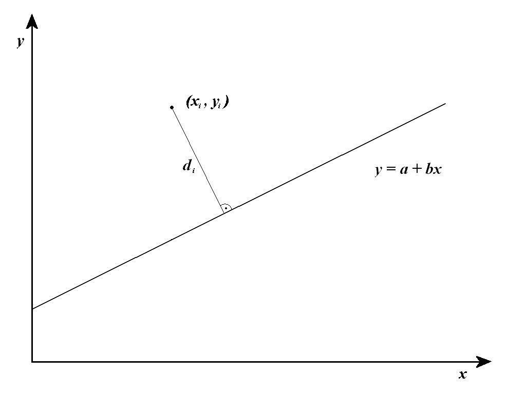
The PCA fitting method involves a mathematical procedure that transforms a number of correlated variables into a smaller number of uncorrelated parameters called principal components. The approach is equivalent to a least-squares fit that minimises the squared orthogonal (i.e. perpendicular) distance of the measured points from a linear function, as illustrated.
The perpendicular distance from the fit is
$$d_{i} = \frac{y_{i} - bx_{i} - a}{\sqrt{b_{}^{2} + 1}}$$
Minimising the sum of the squared distance results in the estimation of the slope and the offset of the best fit being
$${b = - B + \sqrt{B^{2} + 1},\quad\textrm{wit}h\quad B = \frac{1}{2}\frac{{\sum_{i}^{}\left( x_{i} - \overline{x} \right)}^{2} - \left( y_{i} - \overline{y} \right)^{2}}{\sum_{i}^{}{\left( x_{i} - \overline{x} \right)\left( y_{i} - \overline{y} \right)}} }{a = \overline{y} - b\overline{x}}$$

PCA method
When forcing the regression line through the origin (a=0) then the slope of the best fit becomes
$$b = - B + \sqrt{B^{2} + 1},\quad\textrm{wit}h\quad B = \frac{1}{2}\frac{\sum_{i}^{}\left( x_{i}^{2} - y_{i}^{2} \right)}{\sum_{i}^{}\left( x_{i}y_{i} \right)}$$
Low wind speed cut-offs
Generally low wind speeds are excluded from correlations as measurements are more inaccurate at low speeds but also it is better to optimise the fit for the wind speeds at which wind turbines are operating.
Iterative approach to determine a "Site" low wind speed cut off
Assuming the reference low wind speed cut off is set at (for example) 3 m/s we apply a directionally averaged speed up value derived from the correlation between the reference and the site wind speeds to determine equivalent low wind speed cut out at the target mast. This directionally averaged speed up is first derived assuming a speed up of 1, i.e. also excluding all data below 3m/s at the target location. We then take that speed up and apply it to the reference to get an initial equivalent 3 m/s cut off at the target. So if the speed-up is 1.1 then the target cut out will be 3.3 m/s. Then the correlation can be undertaken again based on this new target cut off to derive a new speed-up until the target cut-off wind speed stabilises between iterations. By this approach we iterate towards an accurate target low wind speed cut off for the correlation.
Correlation uncertainty (CalculateUncertainty)
Speedups are derived between the “reference” and “target” mast. The uncertainty in the correlation in each direction sector is based upon the scatter in the correlation between the two masts. The correlation uncertainty is based on the quality of the correlation between the two masts and the number of points in each wind direction sector.
Generally, the better the correlation, and the more points in each direction sector of the correlation will give a lower uncertainty. Differences in exposure can have a big impact on the quality of the correlation.
For multi-mast sites, correlation uncertainties are generally lowest when the “reference” mast is placed in the centre of the site or at a location that best represents the rest of the site. A longer overlapping period between the “reference” mast and the “target” mast will also help lower uncertainties.
When calculating the uncertainty in each sector, we re-average the time series to hourly values thus reducing dependence of the wind speed of one record on the wind speed of the next record.
The uncertainty in each direction sector is weighted using the frequency distribution at the reference mast to give the overall uncertainty. Therefore, if a poor correlation is observed in a low frequency direction sector, it will not greatly affect the overall uncertainty.
It is noted that there is currently no agreed uncertainty calculation method defined for correlations not forced through the origin.
Direction trends
Systematic direction trends between the reference and site measurements can be derived and applied to predict site directions from reference data.
The direction shift between the time series is calculated for each one of 36 direction sectors in the following way:
First, the reference direction time series is binned into direction sectors.
For each time step, the difference is calculated between the direction measured at the site and the reference mast.
For all reference wind directions within a direction sector, the mean of these direction differences is calculated
These mean direction offsets form the ‘Direction trend’.
In scripting direction trends can be applied, if required, to either a reference time series (to generate a synthetic site direction time series) or to a reference wind speed and direction frequency distribution to transform it to be representative of the site directional frequencies.
In Direction Reconstruction direction trends are applied to the reference time series to generate synthetic site time series.
Frequency distributions
This frequency distribution is a multi-dimensional array with three key dimensions:
Direction
Speed
Month
De-seasoning
An annually representative speed-by-direction distribution can be created by collapsing the monthly dimension.
De-seasoning may be applied when collapsing the month dimension to remove seasonal bias. It is the process of taking the weighted mean of the frequencies across each month where the weighting is the number of days in the month. For de-seasoning February is weighted by 28.25 days. You cannot de‑season a frequency distribution if you have a calendar month with no records.
If de-seasoning is false, the overall distribution is the straightforward sum of the monthly frequencies.
Creation of a tab file
On output of a tab file we do the following:
Take a copy of the distribution (so the distribution stored in WFA is not changed)
Calculate the overall directional frequencies for each month
Spread the no direction (and wind speed < 0.5 m/s records) through the directional wind speed bins weighted by the overall directional frequencies for the month
Collapse the monthly dimension of the FD (de-seasoning if applicable).
Write out the speed by direction frequencies in the tab file format.
Scaling a frequency distribution using SpeedupFreqDist and ScaleFreqDistTo
Speed-ups are applied to every wind speed bin of the frequency distribution.
We apply speed-ups as follows:
SpeedUpFreqDist
1. Scale the wind speed bin boundaries by a factor (e.g. 2%):
| 0 | …to… | 0 |
|---|---|---|
| 1 | 1.02 | |
| 2 | 2.04 | |
| 3 | 3.06 | |
| 4 | 4.08 | |
| 5 | 5.1 | |
| 6 | 6.12 | |
| 7 | 7.14 | |
| 8 | 8.16 | |
| 9 | 9.18 | |
| 10 | 10.2 | |
| 11 | 11.2 | |
| 12 | 12.2 | |
| 13 | 13.3 | |
| 14 | 14.3 | |
| 15 | 15.3 |
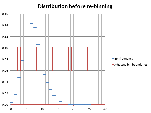
2. Assume a consistent spread of data across each adjusted bin then re-bin the data in to integer bins again by shifting counts accordingly using linear interpolation.
The plot below may help to visualise this: red bars represent the adjusted bins, blue lines are the data in the adjusted bins and the grey gridlines are the bins in to which the data must be re-binned.

To calculate the final wind speed, we collapse the array again along monthly and directional dimensions. This will produce a small discrepancy compared to applying an adjustment to a single overall distribution due to monthly variation in the frequency distribution.
ScaleFreqDistTo
If you want your frequency distribution to match a desired wind speed exactly then use the ScaleFreqDistTo function. This function follows this iterative process:
Scale the frequency distribution in the way described above using the speed-up = (Target wind speed / current wind speed)
Adjusted wind speed is compared to the target wind speed after re-binning the data.
A new speed-up is calculated.
Process is repeated until the frequency distribution wind speed matches the target wind speed to a high degree of accuracy
If this process fails to reach the target wind speed the user is warned
- failure should only happen in extreme cases!