Introduction to WindFarmer: Analyst walk-through exercises

This document outlines how to create a new workbook, run calculations and review the main outputs. Demo data can be downloaded from the customer portal. (Click WindFarmer: Analyst > Documentation > Demo data.zip)

Map

Map setup with online data

Summary: Use the Setup location wizard to set the site location (latitude 20.26°, -longitude 155.875°), co-ordinate system, download elevation data and background satellite imagery.

1. Start a new project

2. In the Project Location task, click 'Start' to start the Setup location wizard

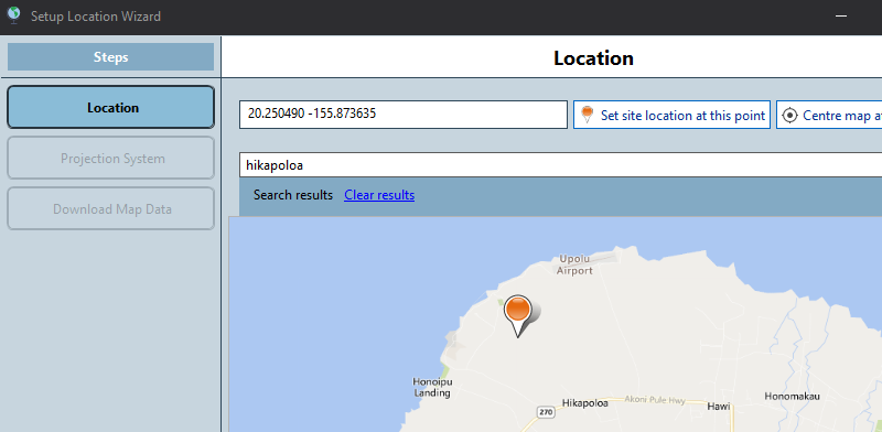
3. Search by name for Hikapoloa and right-click on the map to set the site location (or search by latitude longitude, typing 20.26 -155.875 and clicking 'Set site location at this point'), click ‘Next’

   

4. Use the suggested ‘workbook projection system’: UTM, zone 5 Northern Hemisphere, WGS84. And click 'Next'.

5. Wait for guide background images to download

6. Zoom out by using the mouse wheel or the toolbar button

7. Use the tool to draw a rectangle on the northern tip of the Island

   

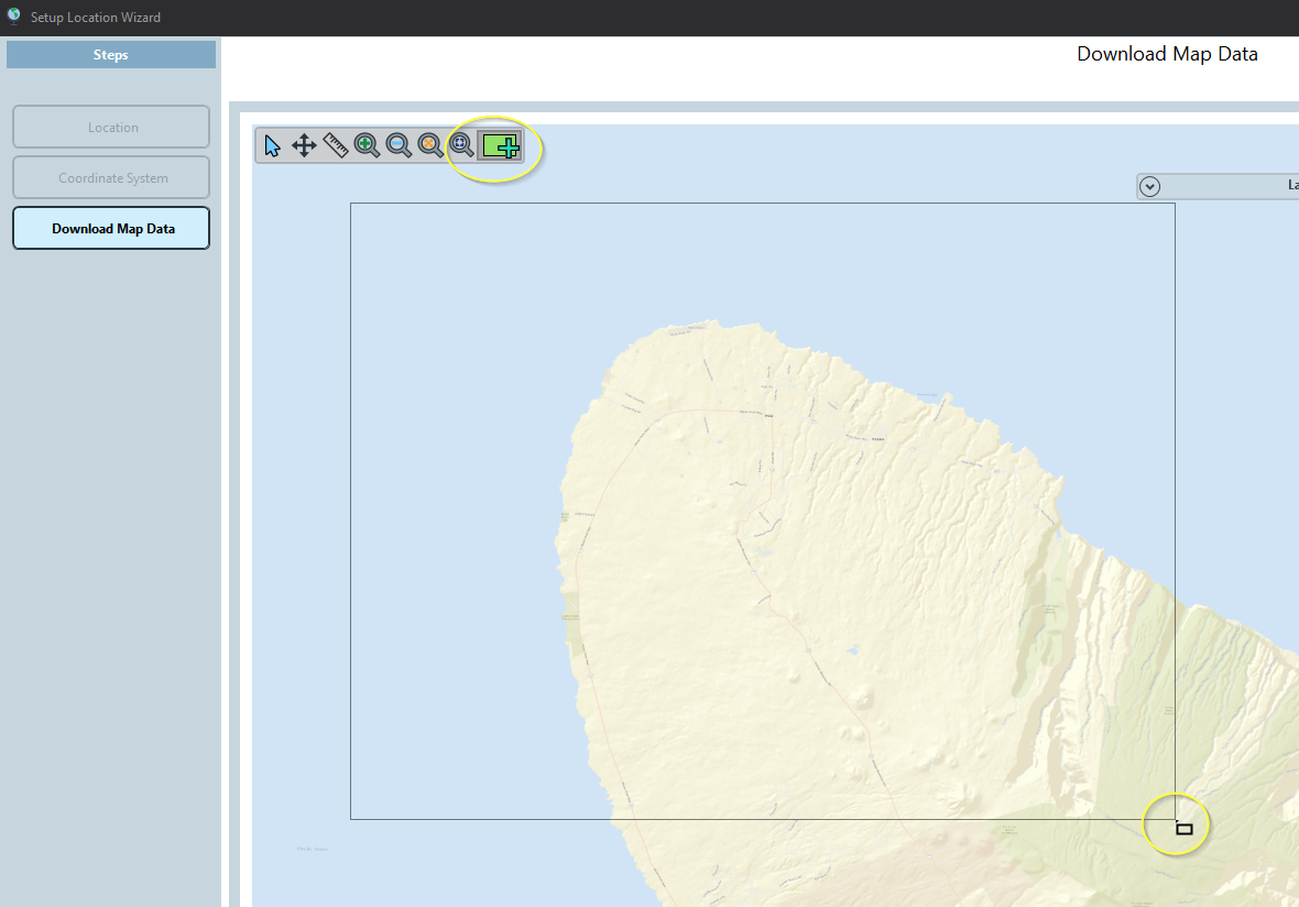
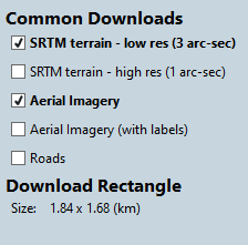
8. Check SRTM terrain, World Imagery (which provides a good satellite image). Then ‘start download’.

   

9. Finish the wizard.

Map setup via file import

Summary: Define the map data in the workbook by importing existing GIS data files from Demo data\GIS data.

1. Start a new project

2. Skip the chapter Map and go to task Background

   

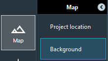
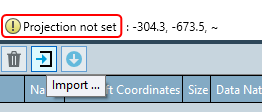
3. Import the background imagery file Satellite imagery.png from the folder Demo data\GIS data

   

Note

The co-ordinate system has now been auto-set because the data had an accompanying '.prj' file.

1. Now import Background image Hawaii.png in the same way. This imagery data is geo-referenced so accept the re-projection on import.

Elevations

WindFarmer: Analyst uses gridded elevations to:

• Derive terrain slopes

• Provide locational height information in the UI and in scripting

Note

If there was no projection '.prj' file accompanying your data, then you will be asked to specify the co-ordinate system on import.

Importing images requires having the accompanying world file next to the image file (e.g. a .pgw file for images in .png format) to automatically convert the image pixels into the metric system used in the workbook

You can download map data without going through the wizard in the Project Location task.

If setting up a map from file, you’ll need to import them here.

To import:

• Import the Elevation contours - Hawaii.map file

• This data is already in the workbook co-ordinate system (UTM, Zone 5, WGS84) but it is not geo-referenced. Accept the assumption that the data is in the workbook co-ordinate system.

• Accept the creation of a DTM to cover the contour area.

You can convert from gridded data (DTM) to contours and visa versa.

Roughness

If you want to run the WAsP flow model within WindFarmer: Analyst you need to import a WAsP '.map' file which contains roughness lines. This '.map' file can contain both elevations and roughness or you can load a separate file for roughness.

Roughness contours can be imported in the Roughness task. They are imported automatically when importing a combined elevations and roughness '.map' file in the Elevations task.

Adjust layer visibility

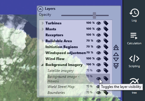
Select layers in the layer control to adjust the layer order, opacity and visibility until you get a mix you are happy with.

Measurement site location

Summary: Define the locations and some properties of measurement sites (Masts, Lidars, Sodars and Reference Stations) used to measure climatic conditions for the project. Measurement sites will hold time series measurements. Here, two masts and a reference staion will be added.

There are three ways to add measurement sites:

1. Paste the tabulated data (e.g. from Excel or tab separated text) in to the measurement site list. You can also find the tabulated data in Excel format in the folder “Mast locations”

   Create two masts and a reference station at the following locations

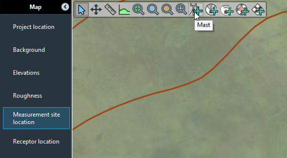
   Type	Name	X	Y
   Mast	M2	202139	2241811
   Mast	M3	199186	2242285
   Reference Station	Kohala Airport	201229	2243339

2. Click to place a Measurement Site on the map by selecting the appropriate toolbar tool:

   

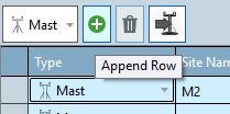
3. Add a Measurement Site by clicking the add button, then fill in the details manually.

   

Note

You can download your masts from Resource Panorama if you are a customer for this DNV service.

Components

Summary: Load in turbine types, either from Demo data\Turbine types or from the library

Turbine types

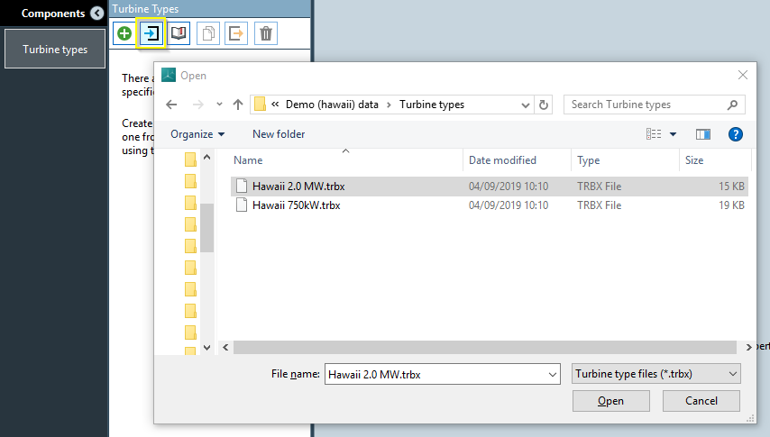
1. Load 2 turbine types from .trbx files in Demo data\Turbine types

   

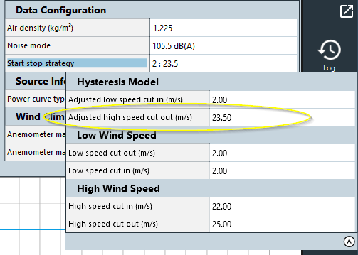
2. Look at the turbine type properties.

3. To model high wind speed hysteresis in later energy calculations, the adjusted turbine high speed cut-out properties are used. For the 2 MW turbine type it is set to be half way between the high wind speed cut-in and high wind speed cut-out wind speeds.

   

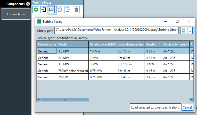
To load a turbine from the library, click the library icon and the Turbine Library window will appear. Select a row and click 'Load selected turbine specifications'.

Wind

Measurements

Summary: Import time series measurements recorded at M2, M3 and Kohala airport from text files found in Demo data\Time series. Define new data loading settings for Mast M2 mapping the columns in the text file to measurement sites, measurements and signals. Load time series data for M3 and Kohala Airport using existing loading settings.

Watch the our tutorial video to see a good overview of the measurement campaign features:

https://renewableenergysoftwareportal.dnv.com/Videos/Play?videoID=3097f546-e063-4aae-a3c6-e7b2c7ab398c

Load measurement data

1. Go to the task Load Measurement data

2. Click ‘add files’

   

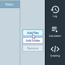
3. Select Demo data\Time series\M2 Time Series.txt.

4. Define loading settings to describe the format of the data. Click ‘New’ to open the settings wizard.

   

Note: If you were loading > 1 file for the mast the selected one is used as a template for defining the settings.

Delimiter and header settings

Here you define the delimitation of the file. In this case the defaults work (it is a tab separated file with 1 line of header).

Click ‘Next’.

Date and Time Settings

Here you need to define the time stamp format. This file has date and time information contained in column 1 so the Combined date and Time option is correct.

1. The time stamp format needs to be changed to yyyy-MM-dd HH:mm. All other settings do not need changing for this file. Note: You can see a preview of how WFA has interpreted the dates to the right:

   

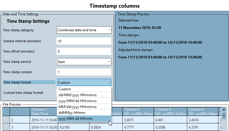
2. Hit ‘next’

Note

Error messages appear at the bottom of the Window and you can’t proceed until the time stamps are interpreted consistently.

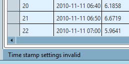
• The Custom time stamp setting can be used to specify almost any time stamp format.

Data columns

The data columns page allows you to assign measurement site and measurement names to the columns of data. The view is transposed for compactness.

1. Type the names of measurement sites and measurements in to the grid in rows corresponding to the data on the right.

   

Note

New measurement sites and measurements will be created if they do not already exist. You can also select measurement site and measurement names that already exist in the project from drop-down lists.

1. To map the time series data file to your measurement site configuration quickly use copy and paste to copy repeated rows to others.

2. To save you time, you can copy and paste (Ctrl+V) selected column mappings to other cells. You can also paste in mappings from excel. See Columns A to C in Demo data\Time series\M2 Sensor Mappings.xlsx for some mappings ready to paste in.

   

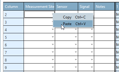
   Rows are shown in blue once the data is mapped.

3. Click ‘Next’.

Measurements and sites

1. In the final step of the settings wizard you can edit properties for each new measurement: name, type, height, boom orientation (if applicable).

2. For convenience, you can also paste in the mappings from columns G to K in Demo data\Time series\M2 Sensor Mappings.xlsx.

   

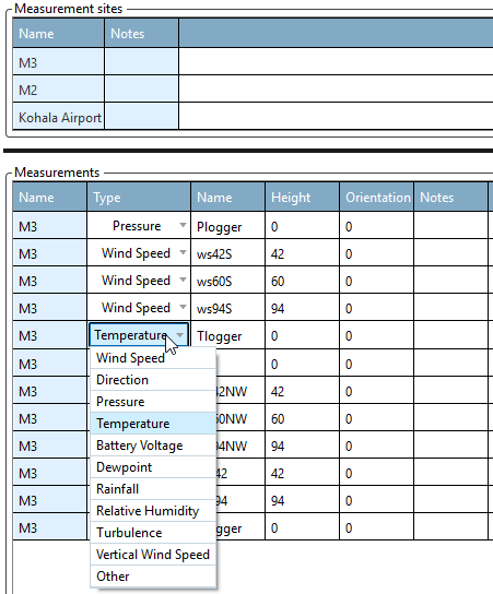
3. Click 'Finish' to complete the settings wizard.

Note

You are asked to save the settings. Settings can be re-used in future sessions to load more data in to the same measurement site or as a starting point for a similar mast.

Also, “M2 time series_LoadSettings WFA.xml” already exists in the Time “series folder”. You can overwrite this.

1. You are now ready to load the time series! Hit Load:

   

2. In the Measurement configuration task you will see a collection of measurements on ‘Mast M2’.

   

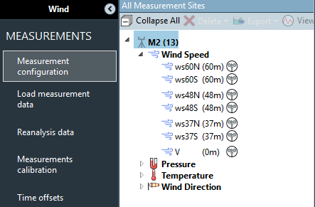
3. In ‘Load Measurement data’, load data for ‘M3’ and ‘Kohala Airport’.

4. Remove the ‘Mast M2’ file from the ‘Load measurements’ user interface,

5. Load data for ‘M3’ with the corresponding settings (click ‘Open’ to select the Mast M3 settings file)

6. Add the ‘reference station time series’ and use its’ corresponding settings.

7. You will need to set the location for these measurement sites. Go to the Measurement site location task in Map chapter and enter in the correct coordinates.

   Type	Name	X	Y
   Mast	M2	202139	2241811
   Mast	M3	199186	2242285
   Reference Station	Kohala Airport	201229	2243339

Note

MERRA or ERA reanalysis data can be downloaded in the Reanalysis data task. This data can be used as reference data in the long term adjustment analysis.

Data cleaning

Summary: Load M3 in to the data cleaner, configure your cleaning workspace. Add extra scatter plots. Exclude clearly erroneous data.

Reference: Watch our data cleaning video found on our website to see an overview of the data cleaning functionality. https://renewableenergysoftwareportal.dnv.com/Videos/Play?videoID=00f016af-168f-443a-8220-d22772a61d49

Note

By default, hardware acceleration is enabled. If you experience a crash, poor performance in the data cleaner accompanied or warnings about your graphics card or your screen going black before recovering your graphics card is likely incompatible with our hardware acceleration. Intel graphics cards commonly exhibit this behaviour. In this case go to File > Preferences and deselect enable hardware acceleration in the Charting tab. After re-starting WindFarmer: Analyst, cleaning will work as expected using software rendering.

You can change to a light theme background for charting if you prefer this by going to File > Preferences then select Chart theme: Light.

Note that excluded data can be hidden from the plots by using the check box in the legend.

In the task Data cleaning, select the data you want to clean from the measurement site tree.

Data can be selected to exclude in the 'Clean Measurements' or measurement site named tabs that show the data as time series. The additional correlation or ratio plots are useful to find any erroneous data, but the exclusions cannot be selected form here. The individual tabs can be moved in the main window and to a second monitor.

Adding exclusions:

To add an exclusion, highlight a time range in the plot and right-click.

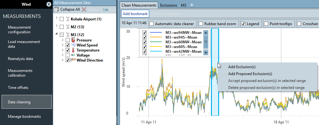
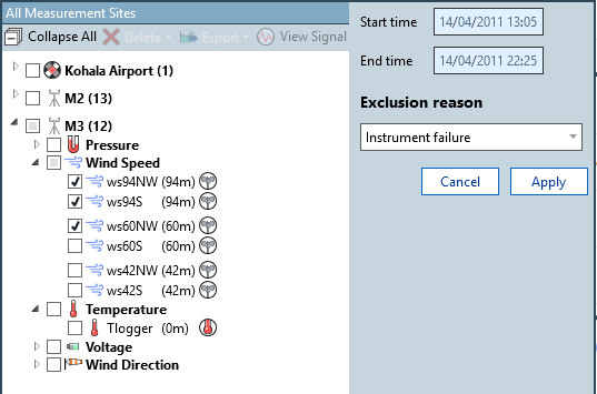
You can either add exclusions (data are not used in any data analysis) or proposed exclusions (data that are only marked but still used in any data analysis). Then select the signals to exclude and the exclusion reason. Click ‘Apply’. Exclusions are show as blue bars, proposed exclusions as orange bars. The exclusions are shown as a list in the ‘Exclusions” tab.

Editing exclusions:

Right click on an existing exclusion and select ‘Edit exclusion(s)’ to edit the time range or exclusion reason. The time range can also be edited by just dragging the beginning or end of the exclusion bars.

To convert proposed exclusions into actual ones, right-click on the proposed exclusion and select ‘Accept proposed exclusion(s)’ from the options. You can also enable the ‘Automatic data cleaner’ option in the toolbar and use the button to accept all visible or all proposed exclusions for this conversion.

Delete exclusions:

Simply click on the exclusion bar and press the Delete key on your keyboard. Exclusions can also be deleted from the list in the ‘Exclusions’ tab.

Reconstruction

In the Reconstruction tasks, the measured time series data are used to generate long-term wind climates for the measurement sites. Those will be one of the inputs into a wind flow model to predict the wind climates at the turbine locations of your wind farm.

In the data reconstruction analysis steps, any reconstruction options with different averaging periods or no overlap with the site data being reconstructed are not shown. (the correlation is not possible).

Note the following features are available in each task:

	Start here in each task. ‘Auto-setup’ selects the default best-practise options based on your data and settings.
	Produce visualisations (correlations, synthesis checks, wind roses etc.) and detailed tabulated results to review the strategy and results.
	Use ‘Re-calculate all’ whenever an input changes. Recalculate all acts over all results calculated within the task so you can quickly update results. ‘Re-calculate’ will not change your existing settings.
	Custom configuration if you need to select inputs not selected by the ‘auto-setup’. (e.g. Reconstruction of a none-primary measurement).

The output time series is automatically saved in the workbook under ‘calculated signals’ under each mast in the side panel:

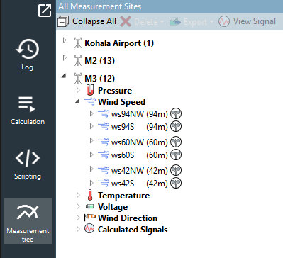
Note

Time series can be exported to as time series, stats files, or visualised with (ctrl + click) then select view signal.

Before executing the analysis steps, ensure:

• Primary wind speed and direction measurements have been selected for each mast in Measurement site configuration. If not selected, the instrument with the largest height is used by default as primary measurement in the auto-setup algorithms.

• Boom orientations have been entered in Measurement site configuration so that parallel measurement combination auto-setup can identify exclusion band centres.

• Representative turbine types are included in to the workbook: these will be used for synthesis checks. See Turbine types in Components.

Direction reconstruction

Summary: reconstruct direction data to increase data coverage for the primary direction signal

Use the auto-setup to automatically evaluate all possible reconstruction options and prioritise those which can fill in any gaps by distance. See how the valid data [years] differs in the input and output series and how many data points from other direction signals have been spliced into the original data. The output time series is labelled ‘D(signal height)_Recon’.

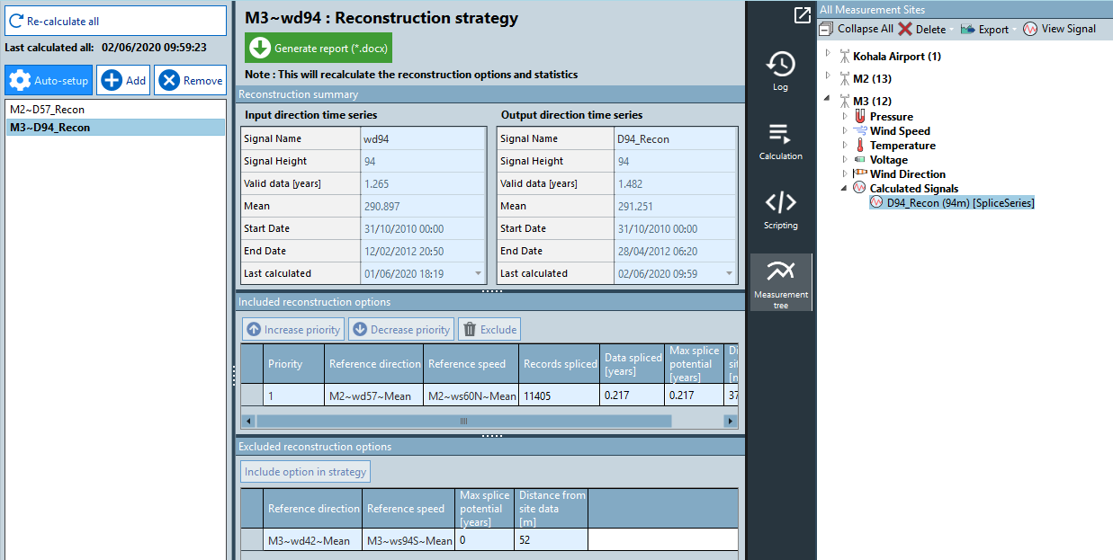
Edit the strategy as you see fit be re-prioritising and excluding options

Use the Generate report button to visualise correlations and review synthesis checks.

Parallel measurement recombination

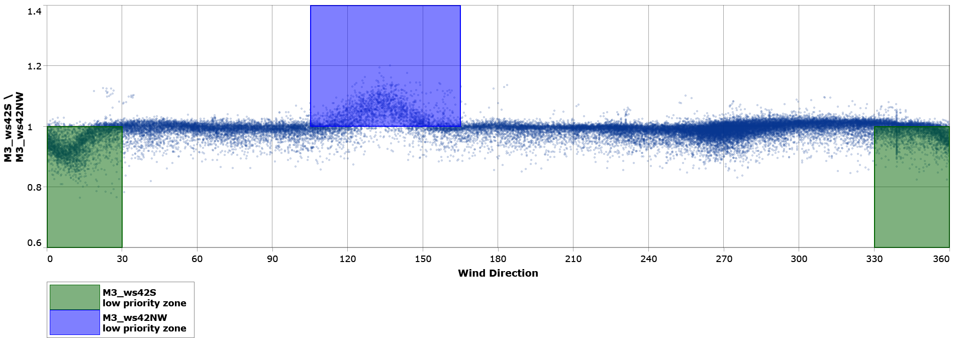
Summary: reconstruct wind speed data to remove mast shadow effects for measurements taken at the same height

Use the auto-setup to automatically splice wind speed data at the same height to remove mast shadow effects. The output time series is labelled ‘PMC(height)’.

Use Generate report button to visualise the parallel measurement recombination results.

Speed reconstruction

Summary: reconstruct wind speed data to increase data coverage for the primary wind direction signal

Use the auto-setup to automatically evaluate all possible reconstruction options and prioritise those which can fill in any gaps by uncertainty. This requires a turbine type to be present in the workbook for the synthesis checks so you need to import turbine type data in Turbine Types in Components. The output time series is labelled ‘Recon(height)’.

Use Generate report button to visualise correlations and review synthesis checks.

Long-term adjustment

Summary: use long term reference data to derive adjustment factors to make data measured on-site representative of long term conditions

The Long-term adjustment task is designed to work with many long-term reference data sets, allowing you to average the adjustments predicted from many sources. Currently there is only one reference data dataset, ‘Kohala Airport’, in the workbook. You can download MERRA 2 and ERA 5 reanalysis data by returning to Measurement Site Setup, ‘Download reanalysis data’. To use our reanalysis data download, you will need to sign in with your Veracity credentials. The reanalysis data for our site in Hawaii will not correlate well with the fake demo data but you could download it to better understand the Long-term adjustment experience.

1. Run the auto-setup and keep all default settings.

2. Select the ‘M2’ and ‘M3’ measurement sites

3. Click on View plot in the ‘Initial Investigations’ table to see the correlation results

   

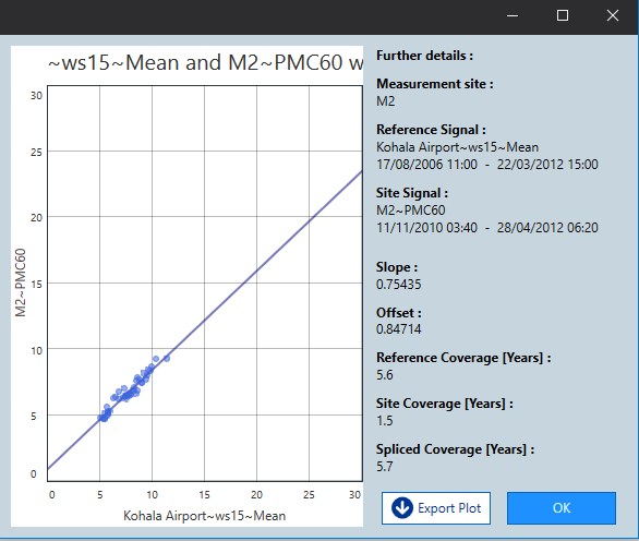
4. Select the adjustment derived from the Kohala Airport reference data to be used as the final adjustment.

   

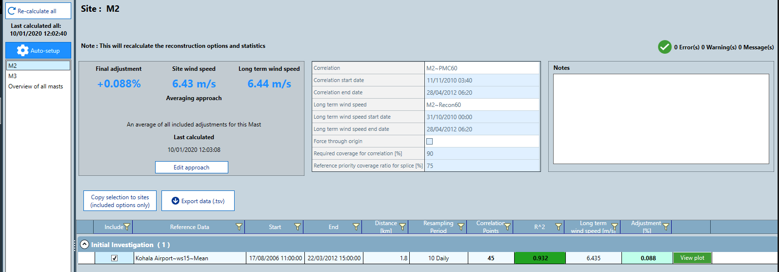
5. Select 'Overview of all masts' to review the adjustments for both measurement sites.

   

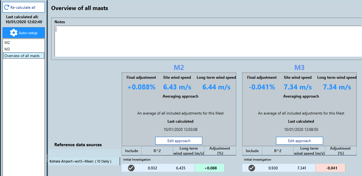
Notes:

When multiple reference data sets are available, results for each source are generated and can be selected to derive an overall adjustment.

Shear model setup

Summary: use wind speed measurements at different heights to define a shear model at the measurement sites.

1. Select each measurement site where you wish to calculate shear and press Edit shear inputs

2. Configure the ‘time series shear model’. Select parallel measurement combined wind speeds, labelled ‘PMC’ and the reconstructed direction data as inputs. Set a hub height, e.g. 100 m, and select the reconstructed wind speed data to be used to in the extrapolation.

   

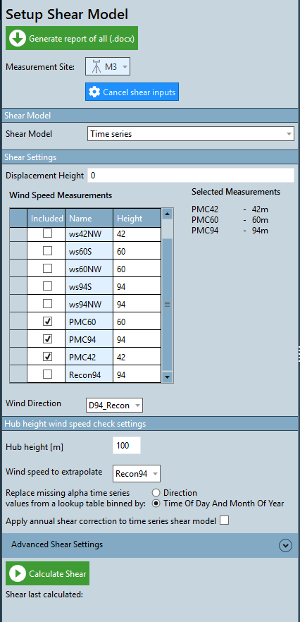
3. Press Calculate Shear and review the plots with the shear model results.

Calculate hub height time series

Summary: generate time series data at turbine hub height based on reconstructed time series data and the shear model.

1. Press Auto-setup.

2. Turbine hub heights are automatically set to those of the turbine types imported in Turbine types in Components. Press OK.

   

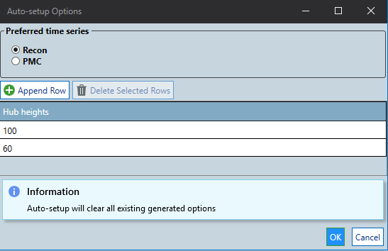
3. Hub height time series data are generated for each hub height and are labelled ‘HHTS(height)’.

   

Calculate wind climate

Summary: generate wind climates based on generated time series data at turbine hub height and long-term adjustments.

1. Run the auto-setup and keep all default settings.

2. Wind climates (wind speed and direction frequency distributions and turbulence intensities) are derived from the time series data at each turbine type hub height and measurement site location. Wind climate data are stored as ‘HHFD(height)’ and ‘HHTI(height)’. This data is used as input in flow model and energy calculations.

   

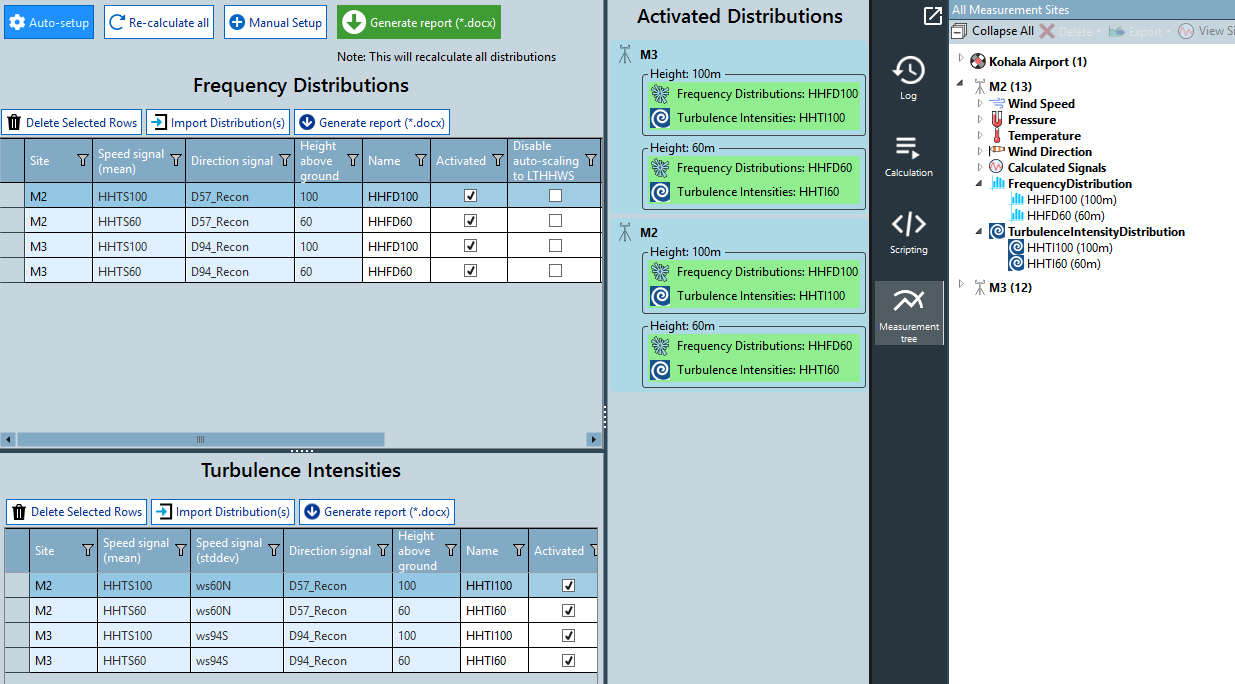
Notes:

We fully support a process where the wind analysis is performed in an external tool and the wind climate data are imported from '.tab' and '.wti' files. See the Appendix: Wind analysis in an external tool for more information on this process.

Flow

There are multiple ways in WindFarmer: Analyst to define the wind flow model and extrapolate wind climate predictions across the site. Depending on your chosen method different actions are needed. You can:

1. WAsP from frequency distribution: Automate WAsP, initiating the model from measurements at Measurement Sites (wind speed and direction frequency distributions '.tab' files)

2. WAsP from wind atlas: Automate WAsP, using a wind atlas to initiate the model (.lib file)

3. Simple flow model with mast specific shear: For quick, indicative studies. Can also be used to quickly generate a uniform wind flow field suitable for some offshore sites.

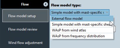
4. External flow model: Import your own flow model (import '.wrg' files at measurement locations and associate with '.wrg' and/or '.rsf' at target locations, or simply import the '.wrg' and/or '.rsf' at target locations alone if you have no onsite measurements)

   

Flow model setup

Summary: set up and run a flow model to predict wind conditions at turbine locations (turbines will need to be placed before flow can be calculated. Go to Design – Place turbines to do this). Alternatively, import flow models from file.

Running the flow model in WindFarmer: Analyst

• When running the ‘flow model’, WindFarmer: Analyst makes no assumptions about assumes the initiation mast for each turbine but calculates from each mast at all target locations so that initiation masts can be analysed and selected later.

• In this example either select “WAsP from frequency distribution” (if you have a WAsP 11 or 12 license and WAsP installed) or the “Simple model with mast specific shear”. Note, if you need to use the ‘simple flow model’ you will need to reset the shear model to “user defined” for M2 and M3 and enter shear parameters manually, defining ‘alpha’ when using the power law or ‘z0’ when using the log law.

• We require a frequency distribution defined at each initiation measurement site, which were defined during wind analysis in the Calculate wind climate task.

By default, WindFarmer will calculate wind flow only at the turbine locations (Discrete predictions).

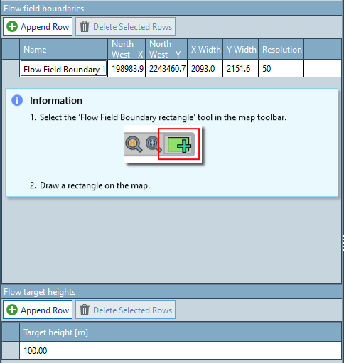
As we will optimise our wind farm layout later on, the region for the turbines in our target wind farm should be generated as a grid.

1. Using the flow Field Boundary tool, draw a rectagle on the map covering the site boundary of our target wind farm where we want to optimise our layout.
2. We also need to select the hub height of our turbines as the 'Target height'.

For the neighbouring wind farm: these turbines have fixed locations so we do not necessarily need to simulate gridded wind flow over the entirety of that area. windFarmer wil automatically calculate these as discrete predictions.

1. Now run the ‘wind flow calculation’.

   

Note

• If you have multiple wind speed and direction frequency distributions loaded on to each mast at different heights WindFarmer automatically initiates the flow model from the distribution at the height closest to the turbine hub height in question. This means that you can model wind shear separately to wind flow.

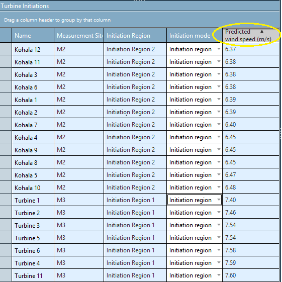
1. Once the ‘flow model calculation’ has completed you can check that results are sensible by looking at the ‘predicted wind speed’ in the Initiations task. Click the header to sort and check no speeds are zero.

   

Importing external flow model with measurement sites

Instead of running a flow model inside WindFarmer, you can import external flow model data. WindFarmer supports ASCII text discrete '.rsf' and gridded '.wrg' files in WAsP format.

Input files:

– Single point '.wrg' file for measurement sites at the height of the measured frequency distribution that was used is input for the external flow model.

– Discrete '.rsf' of gridded '.wrg' files at target height, i.e. hub height. '.rsf' point data must all be for the same hub height.

1. Select ‘External flow model’ as flow model type and press the ‘Import External Flow Model Button’

   

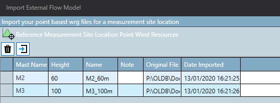
2. Under ‘Import your base point wrg files for a measurement site location, import M2_60m.wrg and M3_100m.wrg from "Demo data\Flow model” as Point Wind Resource. The data is automatically mapped to the measurement sites in the workbook, based on the data coordinates.

   

   

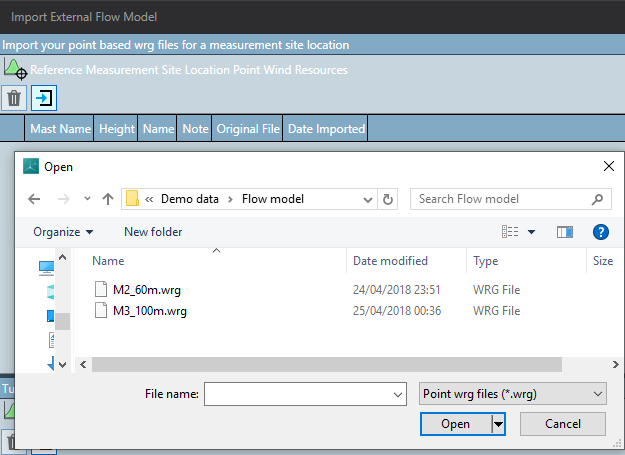
3. Under ‘Import target location wind resources’ import the grid file 100m flow grid from M3.wrg and the discrete resource file M2_60m_Kohala Wind Farm.rsf. Assign the reference location point resources from the dropdown to link the resources at the turbine location with those of the measurement site they originate from.

   

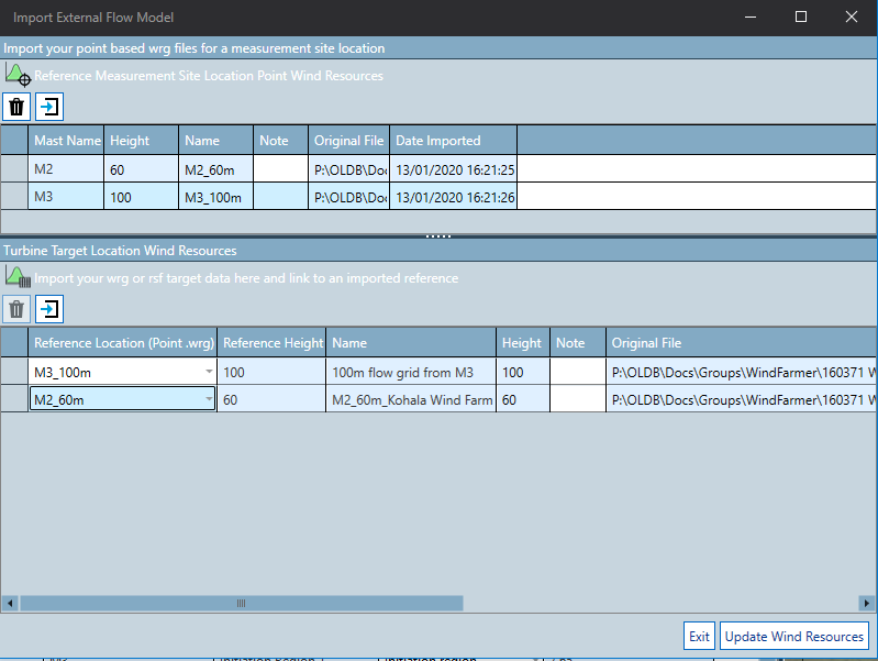
4. Press ‘Update Wind Resources’ to import the data.

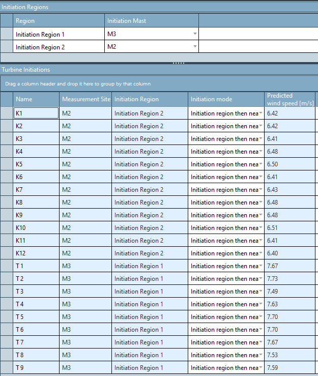
5. In the Turbines Initiations table, ensure that all turbines in the Kohala wind farm use measurement site ‘M2’ and the turbines in the ‘My turbines’ farm use ‘M3’ and have a predicted wind speed value. Depending on the data and the target locations they include, you may have to define initiation regions or a specific measurement site in the ‘Initiation mode’ for the individual turbine locations to clearly define what data is to be used in the energy calculation. By default, WindFarmer assigns the closest measurement site to the turbine locations. When you have imported discrete '.rsf' data that have only one data point per turbine location, you can use the “Auto Generate Initiation Regions”. This feature creates initiation regions based the turbine locations and the available flow model data points.

Wind flow review

Here you can review the data and assignments:

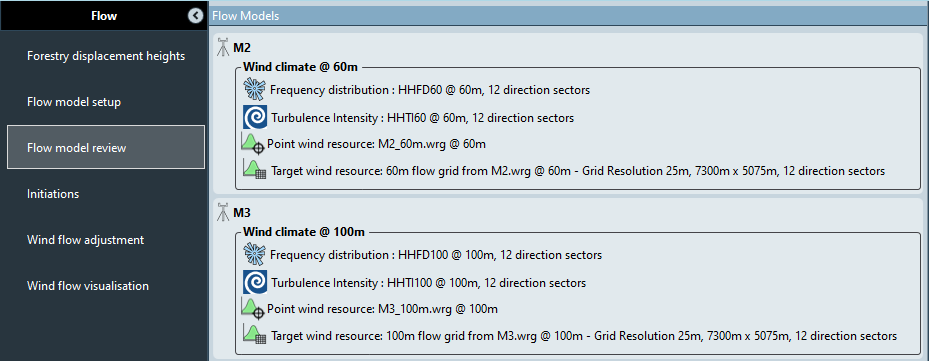
Loaded target wind resources (both calculated and imported files) will also be displayed in a table below

Initiation masts

By default, WindFarmer: Analyst assumes the closest measurement site as the initiation mast for each turbine. We will now make initiations explicit by using an initiation region.

1. Select the initiation region tool

   

2. Draw the initiation regions around the turbines by clicking points on the map. Draw separate regions around the turbines in ‘My Farm’ and ‘Kohala Wind Farm’

   

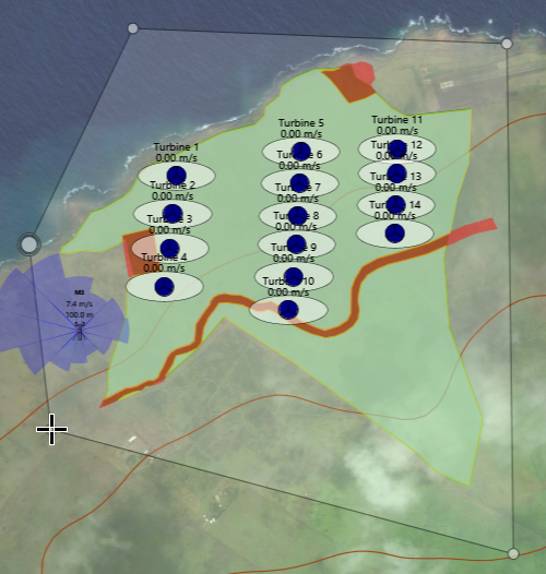
3. To complete the region either double click or click the large circle which was placed at the first point.

   

4. You can then select the mast which initiates turbines within the region. We use either mast M2 or M3 as initiation masts, a good default choice is the closest to the turbines in the region.

   

Wind flow adjustments (optional)

Summary: adjust flow models by applying manual adjustments at turbine locations or regions.

Note

Adjustments can be applied where the flow model is known to underperform, for example you may wish to reduce wind speeds predicted by the WAsP flow model near a steep slope.

By default, no adjustments are applied to the calculated or imported flow model data. Adjustments are applied to all wind direction sectors equally.

There are multiple ways to apply adjustments:

• Based on speedup regions where the same adjustment is applied to all turbines within the region
• Using turbine-specific adjustment factors
• Using turbine-specific target wind speeds
• Wind Flow Calibration applied at all turbine locations

1. In the Manual Adjustments table, select the adjustment mode for the individual turbines and enter a manual adjustment or adjusted wind speed.

   

2. For using speedup regions, add them on the map, using the map toolbar and enter the Region Adjustment in the list of regions. The set the Adjustment Mode to ‘Speedup region’.

Wind flow visualisation

Here you can review the wind flow across the site for a selected direction to better understand what the flow model has predicted.

The wind speeds presented are for a wind speed of 10 m/s at a reference mast. Change the wind direction by rotating the dial.

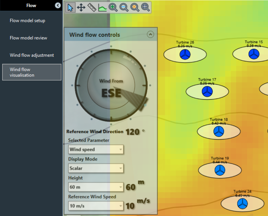
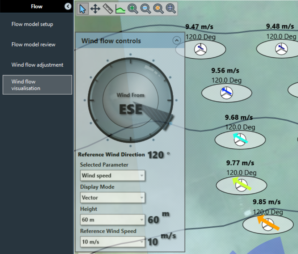
If you have more than one turbine hub height in your project, you can select other heights. There is also a “vector” mode for display of streamlines or arrows. In the case below the “discrete” predictions were calculated (or the user imported '.rsf' files) whereas in the above case “grid” predictions were made (or the user imported a '.wrg' file).

Design

Summary: setup buildable area, wind farms, turbine locations, and optimise your farm layout. Define wind sector & velocity management rules.

Buildable area

Summary: define buildable areas available to place turbines.

If you want to later to optimise your farm you will need to define the Buildable Area, which is the available areas for your wind farm. This can be done either manually by adding inclusion or exclusion regions using the toolbar icons or load those from *.SHP files.

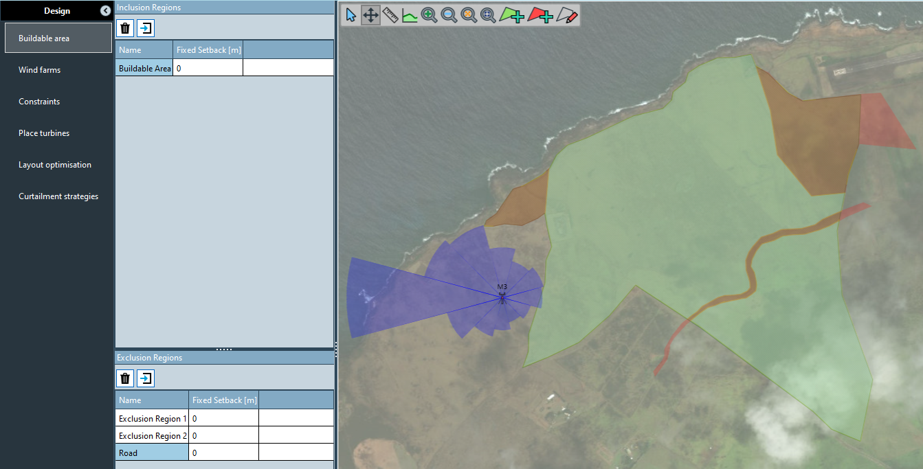
SHP files must include areas that represent your inclusion or exclusion regions. Usage of holes inside areas is supported. Load your SHP files as inclusion or exclusion regions in the panels on the left. The resulting buildable area can be shown by hiding inclusion and exclusion areas from the map layers.

1. Load Boundary.shp as an ‘inclusion region’ from the folder the buildable area from Demo data\Buildable area.

2. Load the other .shp files as ‘exclusion regions’.

Tip

There must be gridded wind flow data available across the entire buildable area at the hub height of the turbine type to be used in optimisation. Go back to the Flow and calculate or import a grid covering the area if this is not the case.

Wind Farms

**Summary: define wind farms. Wind farms is the grouping of turbines. You can easily move turbines between wind farms or exclude a wind farm from a calculation. **

1. Rename the default farm to “My Turbines”. This will be our target wind farm.

2. Add a second farm and call it “Kohala wind farm”. Identify this as a neighbouring wind farm so that energy yield from this farm is not included in a summary of your analysed wind farm. Turbines in this farm will be considered for wake calculations and the wake loss from neighbours is given as an “external wake” efficiency.

Place turbines

Summary: place turbines to define the wind farm layouts to use in flow model and energy calculations

Note

There are multiple ways to define turbine locations (Copy-paste, click on the map, data entry or file import).

Importing turbines from file:

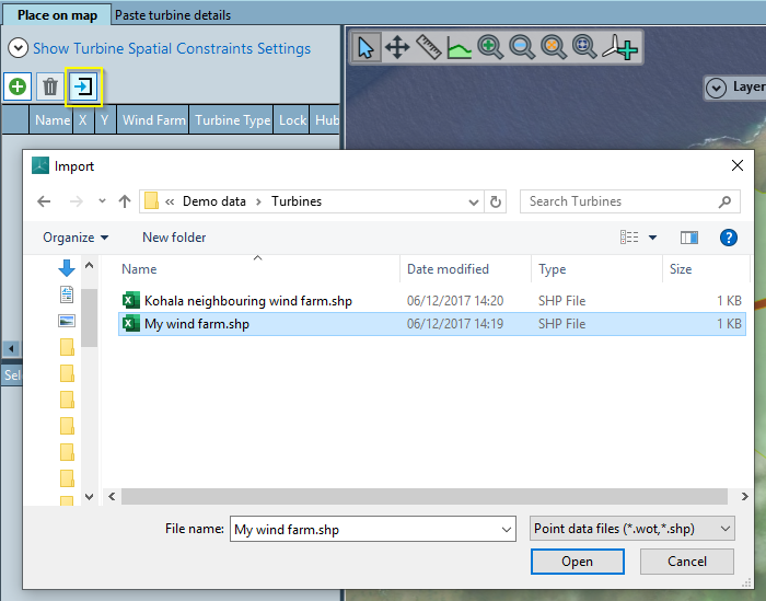
1. Import a shape file “Demo data\Turbines\My wind farm.shp”.

   

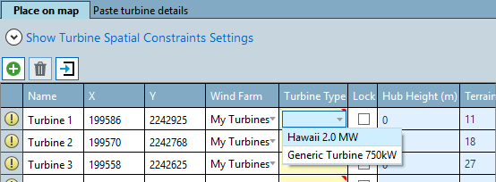
2. Set the turbine type to Hawaii 2.0 MW using the dropdown.

   

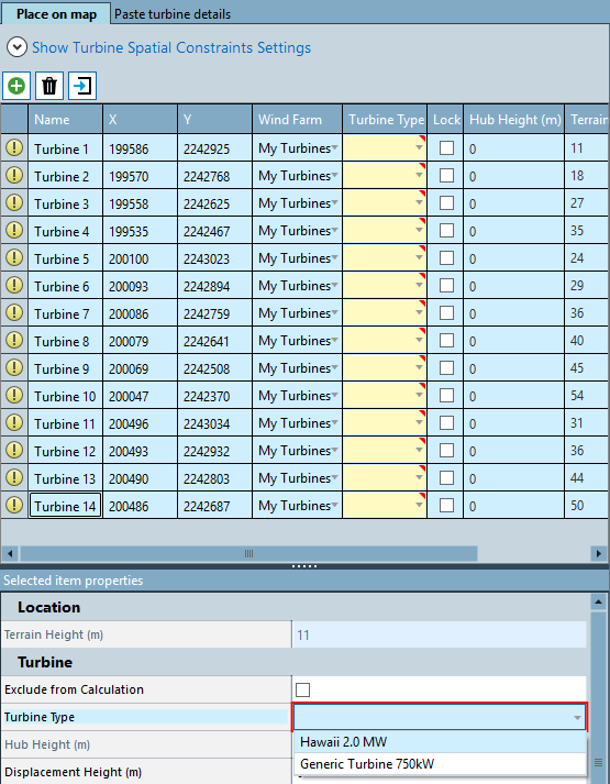
To assign the turbine type for all turbines, select all unassigned turbines by selecting the first turbine (click the grey cell left of the turbine name), holding the ‘Ctrl’ and ‘Shift’ keys on the keyboard, and selecting the last turbine (also by clicking in the grey cell left of the turbine name). Then select the turbine type in ‘Selected item properties’.

![File](../WalkThroughGuide/SetTurbineType2.png)

Paste turbine locations:

1. Open "Demo data\Turbines\Kohala neighbouring wind farm.txt" in a text editor. Copy the file contents.

2. In the table of turbines, select the last turbine and add a new one by clicking the ‘Insert new row’ button. Select the new turbine and paste the data, using the right-click option.

   

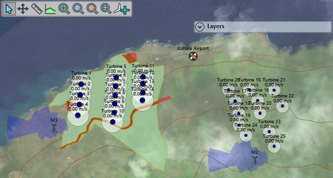
You should now see turbines like the below in the map:

Place turbines directly onto map:

You can add turbines directly in the map.

1. From the satellite imagery (if you downloaded high resolution images) you should be able to identify existing wind turbines in the neighbouring wind farm just south of the airport.

2. Select the add turbine tool in the map toolbar and set the default wind farm and turbine type.

   

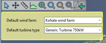
3. Then place the turbines on the map with a left click to create the existing wind farm

Import Turbines

Alternatively, import the “Kohala neighbouring wind farm.shp” file).

Turbine constraints

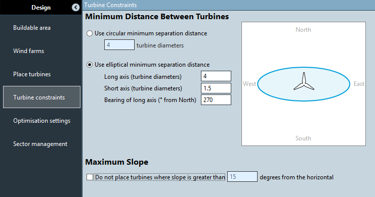
Select the minimum separation distance between turbines as circles or ellipses. This ensures that turbines are not placed too close together to avoid issues with turbine loads due to wake effects.

In this specific case, use an elliptical separation with a long axis of 4 and a short axis of 1.5 diameters and 270 degrees bearing of the long axis. In complex terrain, you may also restrict turbines to be placed on steep slopes to avoid significant upflow effects.

Optimisation settings

Summary: Optimise a wind farm layout, review the layout options and add the best one to the workbook.

1. Before starting to run an optimisation, set the ‘max iterations’ and the ‘number of the top results to keep’ to 10. The random number seed can be used to create a different set of layouts each time the optimiser is run.

   

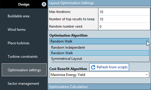
2. There are three different optimisation algorithms available:

   • Random independent: This algorithm places turbines completely randomly so that the start layout and any previously considered layouts are ignored.

   • Random walk: This algorithm considers the previous layout, moving the turbines randomly by a maximum distance that decays with the number of iterations.

   • Symmetrical Layout: With this option, the requested number of turbines is added to the buildable area in a symmetric, row-based layout. The algorithm runs a fixed number of variations for row orientations. This algorithm is suitable whenever symmetric layouts are desired to reduce infrastructure cost, like cables.

   Select ‘Random Independent’ as 'Optimisation Algorithm’ to place the turbines and the ‘Cost Benefit Algorithm’ to ‘Maximise Energy Yield’ to define the target function used to rank the different layouts. In general, you can use the provided options or use your own script to define those.

3. Hit 'Optimisation calculation' to start the optimisation. The results of the top layouts together with the target function results are shown in a table and the results for each iteration are shown in a plot on the left. The optimisation can be stopped from the calculation view in the side bar. The top layouts will be stored in the workbook once the workbook is saved.

   

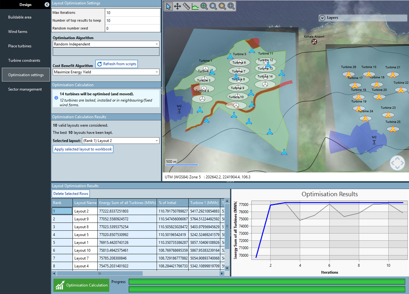
4. After the optimisation is finished, the top layouts can be reviewed by selecting a layout in the results table. The turbine locations are shown in blue.

5. A layout can be applied to the workbook by selecting it from the dropdown list and clicking 'Apply selected layout'. This replaces the initial layout defined in ‘Place Turbines’.

Sector management

Summary: define sector management rules to shut down turbines for specific wind speed and directions to reduce turbine loads, typically done for closely spaced turbines. This will reduce the wind farm energy output.

1. Type or paste in sector management rules for specific turbines in to the ‘Start Direction’ column to specify a rule.

2. To add more than one rule for a turbine, select a row (click box to left of table like you select rows in Excel) then click the ‘insert new row’ button

   

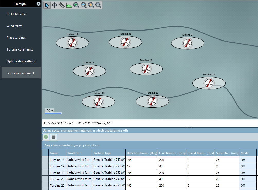
3. Review the defined sector management rules on the map.

Suitability

Design turbulence calculation

The calculation of the design equivalent turbulence to check the suitability of the turbine type for your wind farm is available via the energy calculation.

1. In the next chapter ‘Energy’ under ‘Wake calculation’, you must set in the wake model type to “Modified park” and check ‘Run Design Equivalent Turbulence Calculation’.

   

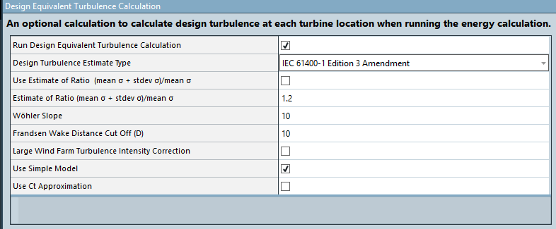
2. The calculation is run by clicking ‘Run Energy Calculation’ in ‘Wake calculation’. Prior to running the calculation, select the matrix channels #10 and #11 to get access to the results. Below is what you’ll see in the ‘Wake calculation’ task.

   

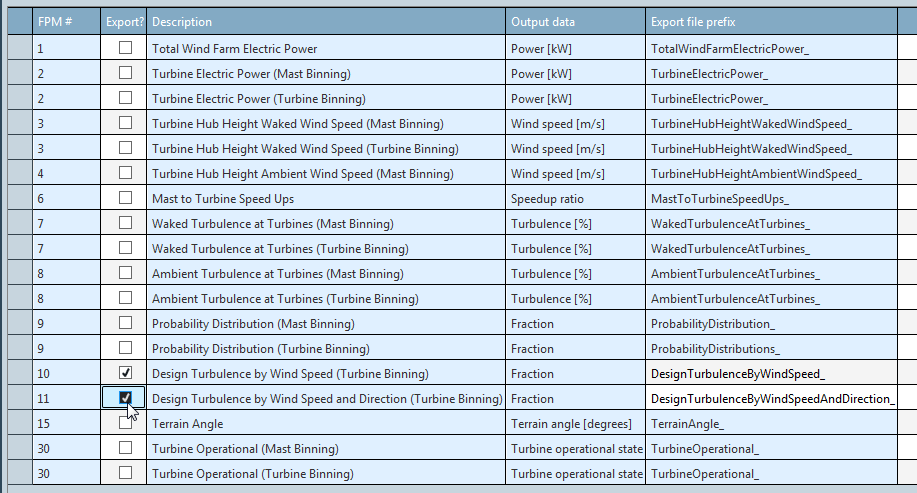
Note

If you defined wind sector management rules you earlier you will get zero turbulence intensity reported in the FPMs for flow cases where your turbines are off.

Energy

Wake and full AEP

Air density

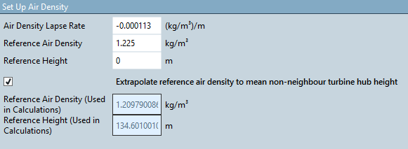
Summary: define the reference air density to correct the turbine type power curve from the manufacturer supplied power curve to one adjusted for the site.

Wake calculation

Summary: Define calculation models and settings for the energy calculation.

Turbine interaction settings and Frequency domain AEP tasks allow the user to define models and settings to use in the energy calculation and to review and export results, once the calculation has been run.

The 'Turbine interaction settings' task allows the user to define large wind farm correction, wake model and blockage model settings which apply to flow calibration tuning, frequency domain AEP and power time series calculation.

Turbine interaction model

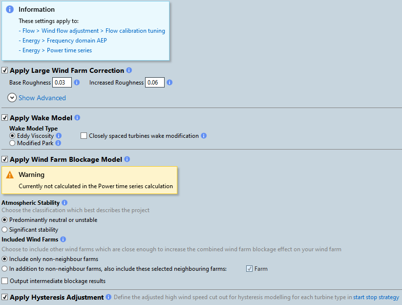
• Apply the Large Wind Farm Correction to consider interaction losses with the free flow inside large wind farms or between wind farm clusters. The base roughness should be equal to the average roughness of the wind farm site following the Davenport convention (also used by WAsP). The increased roughness should be equal to the base roughness + 0.03 in most cases. In some cases of high atmospheric stability wakes decay more slowly and a higher additional factor should be used. Different settings may also be used offshore. DNV regularly validate the WindFarmer wake model to refine the settings used in energy production assessments. If you have WasP available, you may calculate base roughness via scripting.

• Select either the Eddy Viscosity or Modified Park wake model to consider turbine interaction losses due to wakes caused by individual turbines. As the Eddy Viscosity model is more sophisticated, it is recommended to use this in the energy calculation. The Park model is a simpler model that is faster to run so it is recommended to use this when running layout optimisations.

• Apply the Wind Farm Blockage Model to consider effects wind farms have on the upstream ambient flow.

Settings

The 'Frequency domain AEP' task allows the user to define models and settings to use in the energy calculation and to review and export results, once the calculation has been run.

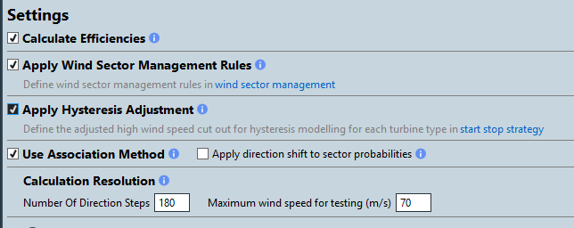
• Check “Calculate Efficiencies”. This will run the energy calculation several times to attempt to quantify turbine interaction effects, the high wind speed hysteresis effect and the effect of wind sector management as efficiencies (a percentage total energy when compared to the gross energy).

• Apply wind sector management rules to consider the rules set in ‘Sector Management’ in the energy calculation. If “Calculate Efficiencies” is enabled, hysteresis sector management effects are reported separately.

• Apply hysteresis adjustment to consider hysteresis adjusted wind speeds for each turbine type. If “Calculate Efficiencies” is enabled, hysteresis effects are reported separately.

• Use the association method to give measured wind speed and direction distributions at measurement sites priority over data simulated by flow models and more advanced wake modelling. This is required for modelling net yield distributions in the ‘Net energy’ task.

• Select the number of direction and speed steps to use in the energy calculation.

Export

• Enable the export of Flow and performance matrices to get access to detailed simulation results. This needs to be specified before running the energy calculation.

• Select an output folder for the FPMs (if it doesn’t exist it will be created) then check each option desired. FPM Data is exported to text files for all turbines in non-neighbour projects once the energy calculation is complete.

Now you are ready to calculate the annual energy production for your wind farm.

• Click ‘Run energy calculation’ in the main view or from the ‘Calculation’ tab on the side panel.

Once finished, results can be reviewed further on in the chapter in the results tasks.

Note

If you defined wind sector management rules you earlier you will get zero turbulence intensity reported in the FPMs for flow cases where your turbines are off.

Net energy

Energy results in the ‘Wake Calculation’ task include effects on the yield that can be calculated with the WindFarmer models. However, there are additional effects to be considered in the final wind farm net yield. When it comes to financing wind farms, the uncertainty in the annual wind farm energy yield needs to be considered, usually described by so-called exceedance levels that define the yield that is exceeded with specific probabilities.

The ‘Net energy’ task allows to define uncertainties and efficiencies and run simulations of the net energy probability distributions.

Uncertainties

Summary: enter uncertainties in the wind speeds, variabilities and energy uncertainties, to model their impact on the uncertainty in the net yield.

Uncertainties can be entered for each wind climate used in the energy calculation. Note that only wind climates that are used for turbines in non-neighbour farms are relevant. In this case this is the climate at 100 m height initiated from the “M3” measurement site.

Annual Variabilities

• Use the defaults for wind speed interannual variability (variation of mean wind speed from year to year) and frequency distribution interannual variability (variation in wind flow energy due to changes in the wind direction distribution from year to year).
• Custom future annual variabilities can also be added.

Wind climate information

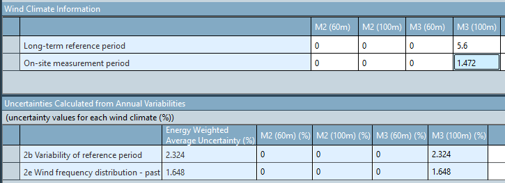
• Enter the number of years as long-term reference period, based on the longest long-term reference dataset used in the ‘Long term adjustment’ task.

• Enter the number of years as on-site measurement period, using what is shown for the wind climate in the ‘Calculate Wind Climate’ task.

• The corresponding uncertainties are automatically calculated from the specified periods and the Annual Variabilities

Wind speed uncertainties

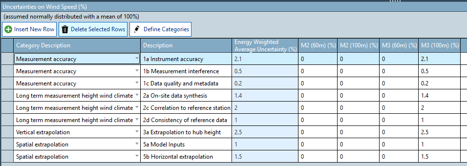
A default list of wind speed uncertainties is provided. You can add and remove uncertainty items from the list and define your own categories. The uncertainties to be considered are site-specific and DNV does not provide recommendations on defaults in WindFarmer: Analyst.

• Enter wind speed uncertainties for each wind climate.

Other energy uncertainties

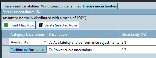
• Enter the uncertainty factors that affect the overall net energy result in this table.

Efficiencies

Summary: define fixed energy efficiencies and their uncertainties to consider additional effects on the overall net energy and its uncertainty.

Note

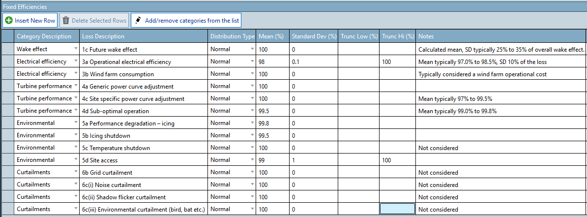
The term ‘efficiency’ is used to define effects on the energy yield instead of the terms “loss” or “gain”. For example, a reduction of the energy yield due to grid curtailment losses of 10% needs to be defined as an efficiency of 90%.

Calculated efficiencies

The mean values of those efficiencies are calculated by WindFarmer: Analyst as part of the energy calculation, if the ‘Calculate Efficiencies’ checkbox was checked. The standard deviation represents the uncertainty of that mean and needs to be specified by the user. Truncation values only need to be added when efficiencies probability distributions should to be limited to a specific range.

Fixed efficiencies

A default list of efficiencies is provided. You can add and remove items from the list and define your own categories. Some general default assumptions and guidance notes are provided for efficiencies and uncertainties (specified as standard deviation) but the user should specify site-specific values.

Time Dependent Efficiencies

Summary: define time-dependent energy efficiencies and their uncertainties to consider additional effects on the overall net energy and its uncertainty.

You can enter time dependent efficiencies for each year for the specified range of years to model. Examples of time dependent efficiencies are drivetrain degradation, affecting turbine performance over the wind farm lifetime or future tree growth that can change the flow.

Net Energy Calculation

Summary: set up and run the net energy simulation

Note

The simulation requires the energy calculation to use the mast association method. When this has not been used, go back to ‘Wake calculation’, tick ‘Use Association Method', then rerun the energy calculation.

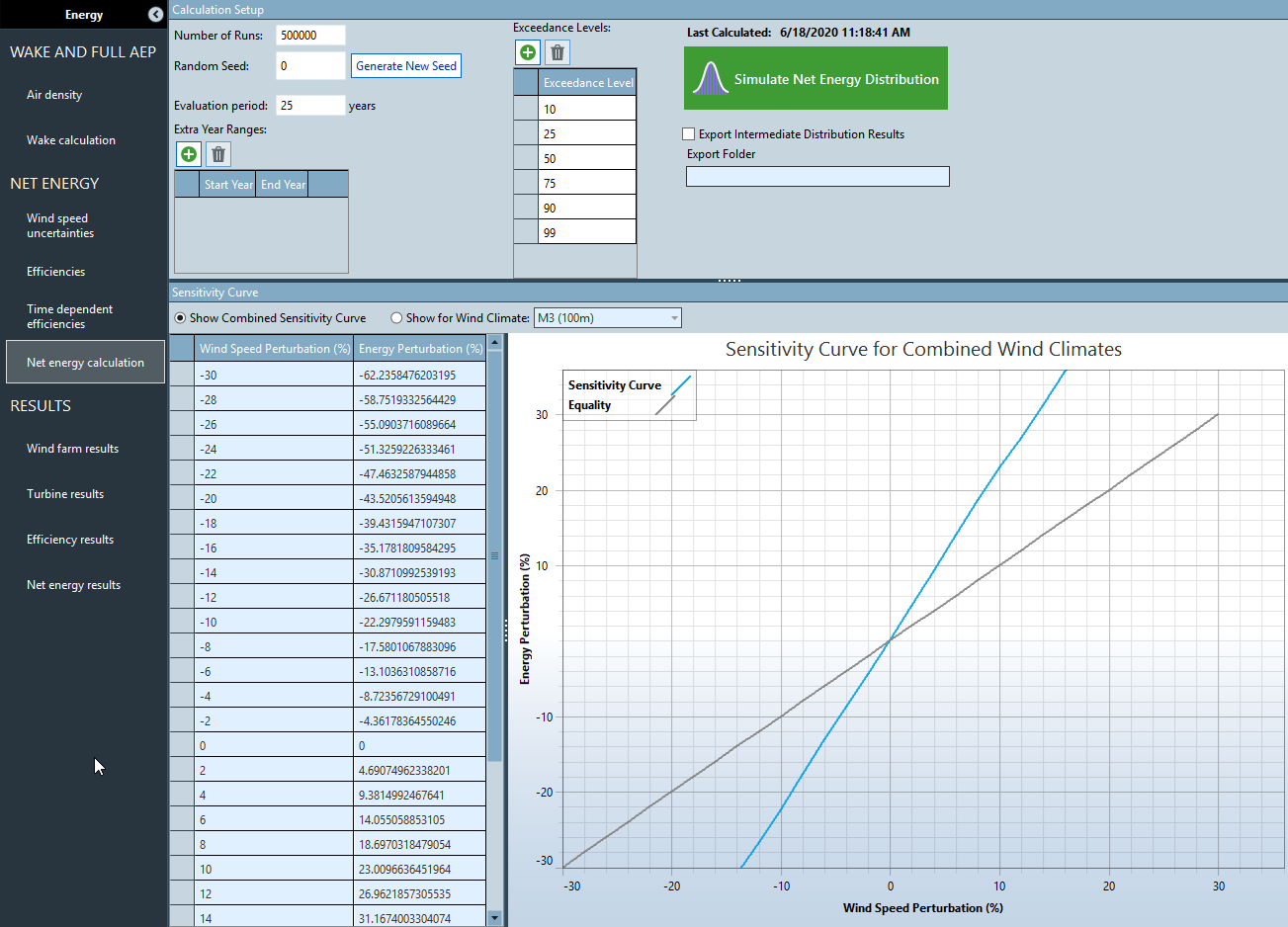
You can add additional year ranges and exceedance levels to simulate and report.

Click ‘Simulate Net Energy Distribution'.

Results

Wind farm results

You can quickly review the energy results for each farm in ‘Wind farm results’.

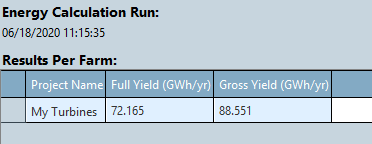
Similarly you can view the results per turbine in ‘Turbine results’ and efficiencies in ‘Efficiency results’.

Net energy results

Once net energy has been calculated, distributions for the entire evaluation period and the individual years are shown. The numbers represent the distribution of the net yield, considering all effects and uncertainties specified by the user.

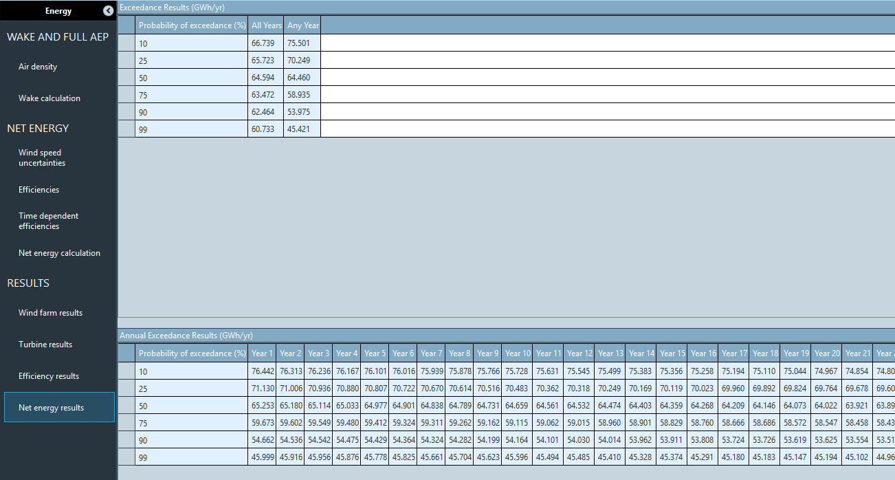
The results can be reviewed more comprehensively in a report that can be generated in the ‘Report export’ task in the next chapter.

Report

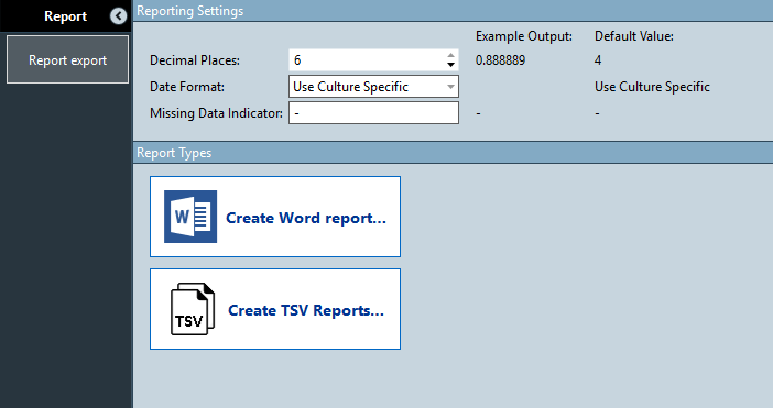
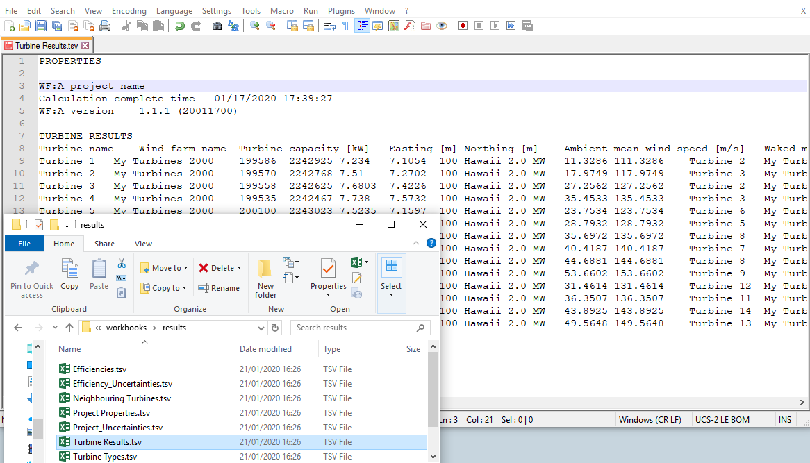
Create Word or TSV reports to review results.

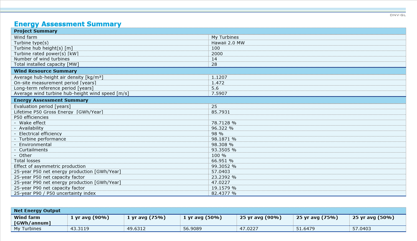
1. Create a Word report to review results from all the modelling steps performed and a summary of the net energy simulation, detailing all the effects considered

   

2. Create TSV reports to review results in a simple tab-separated text format. A selection of reports are exported to a specified folder.

   

Appendix: Alternative Workflows

Wind analysis in an external tool

Wind climate data may be available as external files from other tools. In this case, files can be directly imported here and the data cleaning and reconstruction tasks can be skipped. Demo tab and '.wti' files for import are available from Demo data\Tab and '.wti' files.

1. Click the ‘Import Distributions’ button in the Frequency Distributions table

   

2. Select the '.tab' file for mast M2:

   

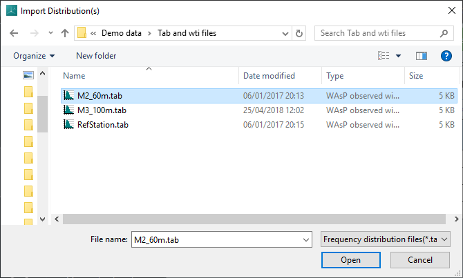
3. Confirm the measurement site assignment and height of data (the height above ground is set to what is in the '.tab' file automatically)

   

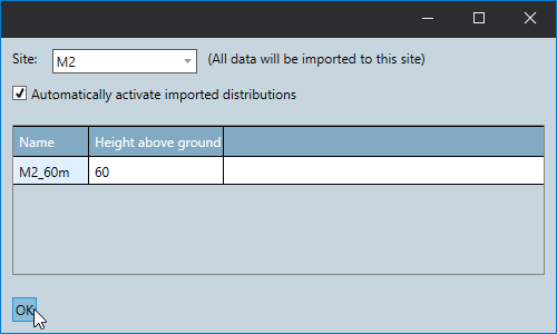
4. Repeat this for the Mast M3 '.tab' file.

5. Do the same for ‘turbulence intensity’ files ('.wti' file) in the ‘Turbulence Intensity’ section of the window. These files do not include height information, so they need to have a height defined. Use the same height as the height for the '.tab' file.

Wind flow model from and external tool with no measurement sites

If you have no onsite measurement data, you can import external discrete and gridded flow model data without requiring a single point '.wrg' file. In this case, a flow reference point will be created at the centre-most point of each imported file.

1. In Flow model setup choose the flow mode type External flow model and click Import External Flow Model **without* Measurement Site*

2. Import the flow data (WRG or RSF file) into the table

3. When you have selected all the data, click on Update Wind Resources. All previously loaded/calculated flow models will be replaced with the new data.

4. Review the imported flow data by clicking the flow model review task. Each loaded wind resource will be seen attached to a flow reference point, and also in a table. From here it may also be easily deleted.

Note

The initiations task is not relevent and can be skipped for this workflow.